
Identification and classification of electrical loads in mining enterprises based on signal decomposition methods
- 1 — Ph.D., Dr.Sci. Head of Department Empress Catherine ΙΙ Saint Petersburg Mining University ▪ Orcid ▪ Elibrary ▪ Scopus ▪ ResearcherID
- 2 — Postgraduate Student Empress Catherine ΙΙ Saint Petersburg Mining University ▪ Orcid ▪ Elibrary ▪ Scopus
Abstract
This study investigates the use of Singular value decomposition to decompose time series of electricity consumption from substation feeders. The goal is to identify and classify the electrical load patterns of mining enterprises. The need for continuous improvement in process efficiency is dictated by current trends and tendencies towards increased consumption of fossil fuels and energy resources. The proposed algorithm uses the decomposition results to identify similarities in consumption patterns, enabling the categorization of loads into broader groups. Based on the results of the analysis of electricity consumption data for two independent feeders, the formation of similar recurring characteristic load changes (temporal patterns) with a period of three days was identified. The results facilitate the automated typification and classification of load profiles. This is vital for integrating economic incentives into demand management and for assessing the feasibility and potential of consumer participation in load schedule regulation via demand side management technologies. The proposed algorithms enable the use of these typical consumption profiles to calculate quasi-dynamic electrical modes, supporting tasks related to the long-term development of energy supply systems and energy efficiency improvements for mining enterprises.

The work was carried out as part of a State assignment from the Ministry of Science and Higher Education of the Russian Federation N FSRW-2023-0002 “Fundamental interdisciplinary research into the Earth's interior and processes of integrated development of georesources”.
Introduction
The need to improve the efficiency of mining operations is dictated by current trends and tendencies, in particular the increase in the consumption of minerals [1-3]. Digital transformation, based on the use of digital technologies and mathematical methods that enable the processing and analysis of large volumes of data generated by mining equipment, improves the efficiency of technological processes throughout the entire mineral extraction chain from geological exploration to resource consumption [4-6]. Similar to the tasks of improving electricity quality [7, 8], methods, based on models of the object under study, must be used to ensure a sufficient level of energy efficiency [9, 10].
The article discusses an approach to improving the efficiency of power supply system to a mining enterprise based on the identification and classification of electrical loads through signal decomposition. Signal decomposition is the breakdown of the original signal (time series) into components represented as modes, components, etc. Signal decomposition methods are determined based on the characteristics of the analysed time series [11, 12] (Table 1).
Table 1
Characteristics of decomposition methods used in power grids
|
Method |
Scope of application |
Disadvantages |
Literary source |
|
Fourier transform |
Harmonic analysis in electrical networks (THD, harmonic distortion). Identification of seasonal components in the load. Detection of equipment faults based on the current or voltage spectrum |
Assumes signal stationarity, which is rarely the case in real loads. Not suitable for analyzing nonlinear and non-stationary processes, which are common in the mining industry |
[13-16] |
|
Singular value decomposition, SVD |
Decomposition of load time series into trend and cyclical components. Signal noise removal. Analysis of non-stationary processes in power grids |
No shortcomings found |
[17-20] |
|
Empirical mode decomposition, EMD |
Analysis of non-stationary electrical loads in mines and quarries. Equipment diagnostics based on vibrations and currents. Improved real-time load forecasting |
The method is prone to modal mixing (different frequencies in one IMF). High noise sensitivity |
[13, 21-23] |
|
Variational mode decomposition, VMD |
Analysis and forecasting of electrical load under variable production conditions. Identification of abnormal equipment operating modes. Joint use with AI models (e.g., LSTM) for forecasting |
Dependence on initial parameters. High computational complexity, problems with processing signals with sharp jumps or pulses. Does not guarantee complete separation of overlapping frequency components |
[24, 25] |
|
Hilbert – Huang transformation(HHT) |
Analysis of transient processes in mining enterprise networks. Diagnosis of faults in electric motors and pumps. Monitoring of electricity quality |
The problem of modal mixing. Edge effects. High sensitivity to noise. Complexity of automation and standardisation |
[26-28] |
Various decomposition methods are used in different technological processes related to energy supply for mining enterprises [29, 30]. The choice of a specific method depends on the volume of data, its statistical characteristics, and other factors that are currently not the subject of this study.
Research involving Fourier transform as a research method is most often devoted to analysing power quality parameters in power supply networks. In the papers of Russian and foreign scientists, the use of singular value decomposition has recently become very popular and is associated with solving a large number of problems. For example, in the study [24], the singular value decomposition method is applied as part of a singular spectrum analysis complex when solving problems of electricity consumption forecasting in an isolated hybrid electrical engineering complex.
Despite the fact that in the mining industry, a significant part of research on the analysis of the condition of electromechanical equipment is based on the use of spectral analysis methods, such as Fourier transform and singular value decomposition, in most cases they are used to diagnose the condition of individual components, such as bearings, or generally to analyze the vibration characteristics of the equipment. At the same time, the influence of the structure and parameters of the electric drive, including the type of motor, control system, operating modes and interaction with the technological process, on the nature of electricity consumption from the grid remains insufficiently studied. This limits the possibilities for comprehensive analysis of electrical modes and reduces the accuracy of load forecasting, especially when using adaptive signal analysis methods. Thus, in further research, it is advisable to take into account not only the external manifestations of signals (vibration, current, voltage), but also the internal parameters of the electric drive that affect the formation of load in the power grid of mining enterprise.
Methods
Signal decomposition methods are essential analytical techniques used in various disciplines, including complex signal processing, data analysis, and engineering, to extract meaningful components. Well-known methods include Fourier transform, SVD, EMD, and multi-scale singular value decomposition (MSVD) [31, 32], VMD, HHT. These methods provide valuable information about signal characteristics when dealing with problems such as nonlinearity, non-stationarity, noise, and multimodal data, making them indispensable tools in modern analysis. The areas of application of these methods vary and have their own characteristics when applied to different types of problems.
SVD is a fundamental method of linear algebra that allows a matrix to be decomposed into three components, revealing the internal properties of the original matrix. This method is widely used for dimensionality reduction, noise suppression, and data compression in various fields, such as image processing and machine learning. SVD is particularly effective for revealing hidden structures in data, allowing us to understand underlying patterns and relationships. However, this method is sensitive to data outliers, and the decomposition of large matrices must be carried out with considerable computational resources in mind.
EMD is a data-driven method that breaks down a signal into intrinsic modes (IMF) that reflect different frequency components of the signal without relying on predefined basis functions. This method is particularly effective for analyzing non-linear and non-stationary signals, making it suitable for use in condition monitoring and other areas. The EMD process includes a screening algorithm that iteratively extracts IMF from the original signal until the remainder has no apparent variations. In recent studies, the EMD method has been extended to bi-dimensional empirical mode decomposition (BEMD), allowing it to be applied to two-dimensional signals and images.
VMD is a relatively new method aimed at decomposing a signal into a set of frequency-band-limited eigenmode functions. It eliminates some of the limitations of EMD and SVD by applying a variational approach that optimally separates modes based on their own passband frequencies. This method is particularly useful for signals with closely spaced frequency components and provides improved performance in carrier frequency estimation and signal analysis.
HHT combines EMD and Hilbert transform to provide time-frequency analysis of signals. By applying the Hilbert transform to the IMF obtained using EMD, HHT allows the generation of a Hilbert spectrum that shows the instantaneous distribution of signal frequency and energy over time. This approach is particularly effective for analyzing complex signals with time-varying characteristics.
General limitations and selection criteria for any method:
- Non-stationarity and non-linearity. Many real signals have non-stationary and non-linear characteristics. The presence of these characteristics can complicate the analysis and interpretation of signals. Traditional signal processing methods often assume that signals are stationary, which leads to inaccurate conclusions when applied to non-stationary data.
- Noise and data outliers are another serious problem in signal processing. They can distort the true signal and lead to unreliable results. Decomposition methods help solve this problem by isolating meaningful signal components from noise.
- Resolution and feature extraction. Signal decomposition methods also aim to improve their resolution, allowing more information to be extracted. Methods such as discrete wavelet transform (DWT) increase frequency resolution while reducing time resolution, providing a comprehensive representation of the signal at different scales.
- Multimodal data processing. In modern signal processing applications, there is an increasing need to analyse multimodal data that combines different types of signals. Signal decomposition methods facilitate the effective combination of these modalities, improving classification efficiency and allowing for a more complete understanding of the underlying processes.
To obtain the components of the original time series of electricity consumption, it was decided to use the SVD method due to its stability with regard to noisy data. The method also allows processing non-stationary signals (such as the time series under study) by extracting the trend component.
In accordance with the singular analysis method, it is necessary to obtain a trajectory matrix from the initial time series. To do this, the initial time series, which has N values {p1, …, pN}, is embedded in a space with dimension L. In Russian literature, this method of obtaining a trajectory matrix from a time series is called “Gusenica” (eng. Caterpillar), while in foreign literature it is called Embedding. The value L determines the dimension of the trajectory matrix and is called the window length. The procedure for determining the window length is a separate scientific task, but when considering time series with known periodicity, the window length is selected based on the duration of the known period. For example, when analyzing the dependence of solar radiation on time over a weekly cycle, it is advisable to set the window length to be equal to, or a multiple of, one day (the period of the observed cycle). In other cases, additional calculations are required to determine the optimal window size.
The result of embedding a time series into an L-dimensional space is an Ln-dimensional (trajectory) matrix (the Hankel matrix):
where p1, p2, …, pn – values of the time series at times t = 1, 2, 3, …, N; n = N – L + 1 – number of columns in the matrix (the number of lagged vectors); the number of rows is the window length and must satisfy the condition L≤[(N+1)/2].
According to [33] any matrix can be represented as:
where matrix U consists of the left singular vectors, i.e. columns of the matrix U consist of the eigenvectors of the matrix AAT; matrix V consists of the right singular vectors, i.e. the columns of the matrix V consist of the eigenvectors of the matrix ATA; σN – singular values of the matrix AAT ( σ=√λ, λ – eigenvalue of the matrix AAT), singular values are located on the main diagonal in descending order.
Let us assume that λ1...λL – eigenvalues of a matrix AAT, at the same time λ1≥λ2...λL. We will also assume U1...UL as columns of a matrix U, taken in accordance with singular values λ.
If we write Vi=XTUi/√λi at the same time i=1, ..., rank(A), then the singular value decomposition of matrix A can be written as follows:
where Ai=√λiUiViT
Each of the matrices Ai has rank 1, so they can be called elementary matrices. Each of √λi,Ui,Vi is called the i-th singular triplets.
At the final stage of the algorithm, each of the matrices Аi obtained from the decomposition is converted back to the form of the original object. This operation is performed by means of matrix Hankelisation (diagonal averaging),
Using diagonal averaging of the components from the obtained matrix, we reconstruct the time series. Thus, the original series is decomposed into the sum of the reconstructed components.
The research [34] presents an original study of time series of electrical energy consumption. This study used graphs of electrical loads of eight substation feeders over a year of observation. The data was obtained directly from the electrical energy and power meter Mercury (a commercial meter with an accuracy class of 0.5). The time series has a sampling interval of 30 min, i.e. the power consumption values are averaged over a 30-minute period.
The original time series consists of 17,520 points. The entire data set includes 140,160 values, which corresponds to the number of feeder connections at the substation. A segment of the original time series for the first feeder, shown on a monthly time scale, is plotted as the purple curve in Fig.1. The results of the SVD decomposition are also shown as the first 12 components reconstructed from the original time series.
Before applying any mathematical transformations, the data was normalized using the min-max method. The original time series was intentionally not pre-processed to remove noise or outliers, to test the algorithm's robustness to input data quality.
Algorithm implementation
The entire algorithm was implemented in the Jupyter Notebook development environment using Python. Aside from auxiliary steps such as importing libraries and defining functions, the main stages of the algorithm are as follows:
- Data import and pre-processing for further analysis. Creating a Pandas DataFrame containing timestamps and power consumption values for each feeder.
- Feature engineering based on datetime data: creating new columns for the day of the month, day of the week, month, quarter, etc. This step is necessary for subsequent data aggregation and dependency analysis across different time periods.
- Performing preliminary correlation analysis by calculating Pearson correlation coefficients (Fig.2). This is used to determine the linear relationship between feeders through pairwise comparison.
- Setting the window width L. When analysing the entire year, the window width is set to Lyear= 1460 data units. based on the average number of points per month. When considering the scale of a month, the window length was defined as the amount of data per week, i.e. Lmonth = 336. Similarly, when considering a single week, the window size was set to Lweek = 48 in accordance with the amount of data per day.
- Creating a trajectory matrix for a single feeder (Fig.3).
- Singular decomposition of the previously created trajectory matrix, verification of the correctness of the decomposition by summing all elementary matrices and then comparing the result with the original matrix.
- Calculation of the relative and cumulative contribution of components to the initial time series for subsequent determination of the required volume of components when grouping them (Fig.4).
- Time series reconstruction. Each elementary matrix is transformed back into a one-dimensional time series component through diagonal averaging (a process also known as Hankelization). The resulting reconstructed components are saved to separate files for subsequent analysis.
- A W-correlation matrix is constructed to quantify the dependence between the reconstructed components. The components are reordered along the matrix's main diagonal according to their contribution (measured by their singular values) to the total variance of the original time series.
- Components are grouped into interpretable modes based on the analysis of the W-correlation matrix. This grouping reveals consumption patterns for each feeder (Fig.5).
The W-correlation matrix reveals a high degree of correlation between specific pairs of components. These components are grouped together based on their strong correlation. For example, a distinct group is formed by components (2, 3, 5, 6), while another group comprises components (3, 4, 7, 8, 11, 12).
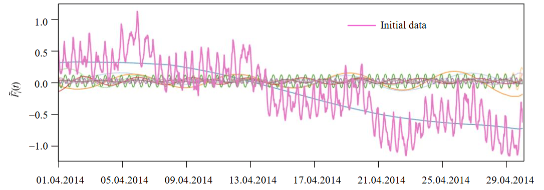
Fig.1. Electricity consumption graph for April 2014 and 12 components of the time series [34]
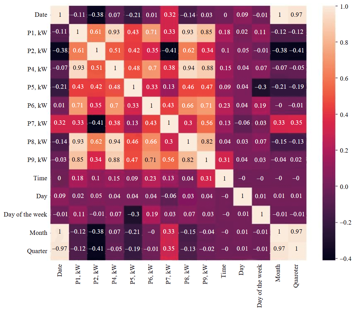
Fig.2. Correlation matrix of initial data using Pearson's method
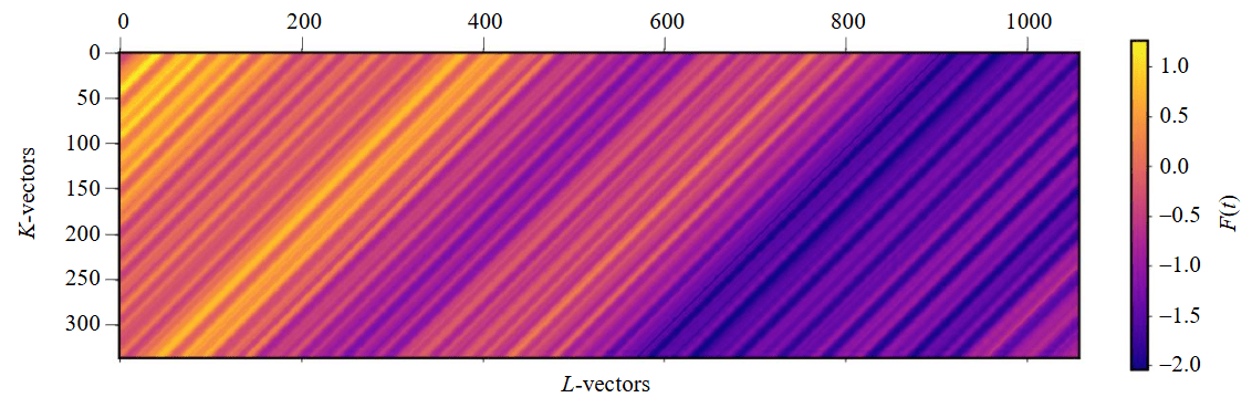
Fig.3. Trajectory matrix of normalized initial data. The time series of feeder 1 is represented as a matrix
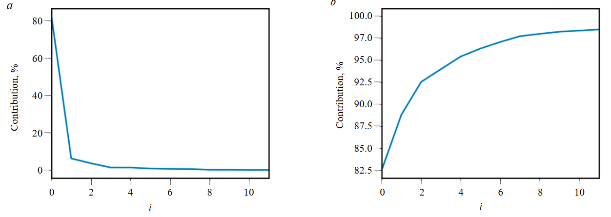
Fig.4. Relative (a) and cumulative (b) contribution of components using the example of a feeder 1
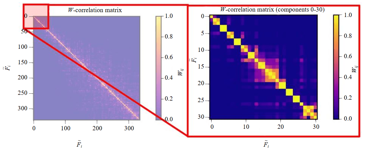
Fig.5. W-correlation matrix for feeder 1 [34]
Results
The study [34] contains the results of manual component grouping using the W-correlation matrix (Fig.6). In this paper the principle of grouping based on the W-correlation matrix was extended using amplitude-frequency clustering and taking into account multiple feeders (Fig.7). For feeder 1, within the time interval under consideration, the components were grouped as follows:
- trend group: 0;
- periodical group 1: 1, 2, 5, 6, 9, 10;
- periodical group 2: 3, 4, 7, 8, 11, 12;
- periodical group 3: 19, 20, 21, 27, 28, 29.
The trend group is characterised by a weekly pattern in the consumption power graph. At the same time, when looking at the original time series, this pattern is difficult to discern.
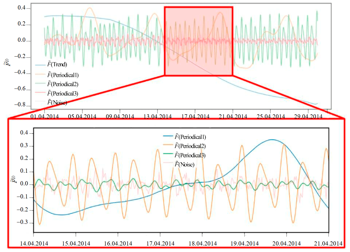
Fig.6. Grouped components of a time series: one trend component and three groups of periodic components [34]
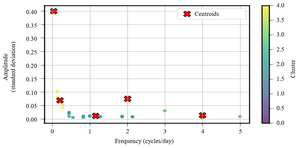
Fig.7. Clustering by frequency and amplitude of the first 10 components of eight feeders
Periodical group 1 is characterised by a daily consumption pattern with strong morning and evening peaks. However, the shape of the curve remains unchanged even with significant changes in the nature of the power consumed and an increase in noise levels.
For periodical group 2, a pattern is formed with a period of occurrence twice a day. The pattern visually resembles a daily one, but the amplitude of its maxima is several times smaller.
The given example is valid for feeder 1 when considering a monthly volume of data. However, the formation of distinct patterns with a certain periodicity holds true for each of the datasets considered in the study. Furthermore, the patterns are unique for each feeder and vary depending on the type of connected load. Table 2 presents the analysis results for the entire dataset.
Based on the assumption of constant frequency and amplitude of a component over the entire segment under consideration, an amplitude-frequency plane was constructed. In this plane, the vertical axis represents the RMS value of the component, and the horizontal axis represents the frequencies calculated using the Fourier transform. As a result of analyzing the feeder components using this method, a family of points was obtained on the plane, where each point represents an individual feeder component (Fig.7).
Table 2
Results of applying the SVD method and grouping components via the W-correlation matrix
|
Feeder |
Component |
Characteristic |
Group |
Description |
Note |
|
9 |
0 |
Trend |
0 |
– |
Formation of a daily pattern. Deviant values are determined by a drop in consumption over a period of 1.5 h on Thursday, 17 April 2014, in the middle of the day. The power graph does not depend on the day of the week |
|
1 |
Period – half a day, the maximum matches the morning peak |
1 |
Formation of daily consumption pattern |
||
|
2 |
1 |
||||
|
3 |
Period – one day for both components. Strong mutual W-correlation |
1 |
|||
|
4 |
1 |
||||
|
5 |
– |
2 |
The formation of a harmonic component with a frequency of 3.5 times per day is characteristic |
||
|
6 |
– |
2 |
|||
|
8 |
0 |
Trend |
0 |
– |
Minimum consumption in the evening period, reaching its first peak at midnight. A decrease in consumption is observed at midday |
|
1 |
Period – one day, the maximum matches with the morning period |
1 |
Formation of daily consumption pattern |
||
|
2 |
1 |
||||
|
3 |
Period – half a day, the maximum matches at noon and midnight |
1 |
|||
|
4 |
1 |
||||
|
5 |
– |
2 |
Formation of a harmonic component with a frequency of three times per day |
||
|
6 |
– |
2 |
|||
|
7 |
0 |
Trend |
0 |
– |
Formation of a pronounced daily pattern with recurring sections during the daytime on weekdays, which were separated into a separate pair of components 7 and 8 |
|
1 |
Period – half a day, the maximums match the consumption peaks |
1 |
Formation of daily consumption pattern |
||
|
2 |
1 |
||||
|
3 |
Period – one day, the maximum matches the daily peak load |
1 |
|||
|
4 |
1 |
||||
|
5 |
Period – 1/3 of the day, the maximum matches midnight |
1 |
|||
|
6 |
1 |
||||
|
7 |
Period – 1/5 of the day, the maximum matches with 11 p.m. |
2 |
The amplitude varies depending on the day. On weekends, the amplitude decreases to 0 |
||
|
8 |
2 |
||||
|
9 |
Period – 1/4 of the day, the minimum matches midnight |
3 |
The amplitude and frequency vary slightly within narrow limits depending on the day of the week |
||
|
10 |
3 |
||||
|
6 |
0 |
Trend |
0 |
– |
Formation of an electricity consumption curve that remains virtually unchanged over time. There is no visible daily pattern. On weekdays, consumption ranges from 800 to 1000 kW. On weekends, the values exceed these limits |
|
1 |
0 |
– |
|||
|
2 |
Period – half a day, the maximum occurs at noon and midnight |
1 |
Contrary to expectations, the group does not form a daily pattern. The frequency and amplitude of the group varies widely |
||
|
3 |
1 |
||||
|
4 |
The component correlates weakly with the trend |
0 |
– |
||
|
5 |
Period – 1/4 of the day, the maximum matches midday |
2 |
The component group generates oscillations with an amplitude of less than 3 % of the base signal with a stable frequency and an amplitude that varies within wide limits |
||
|
6 |
2 |
||||
|
7 |
2 |
||||
|
8 |
2 |
||||
|
9 |
Period – more than 1/7 of the day, the minimum matches midnight |
3 |
The component group forms the high-frequency harmonic component of the signal |
||
|
10 |
3 |
||||
|
5 |
0 |
Trend |
0 |
– |
Formation of a daily pattern. Consumption depends on the day of the week: on weekends, the daily pattern disappears. The increase in energy consumption is concentrated in the daytime and evening hours. There is a characteristic drop in energy consumption between 1 and 2 p.m. The amplitude of all components and component groups considered falls to zero on weekends |
|
1 |
Period – one day, the maximum matches the daily peak consumption |
1 |
The component group forms a daily energy consumption pattern. It can be used to classify the type of load as a component group, purified from noise |
||
|
2 |
1 |
||||
|
3 |
Period – half a day, the maximum matches at noon and midnight |
1 |
|||
|
4 |
1 |
||||
|
5 |
Period – 1/4 of the day, the minimum matches midnight |
2 |
The component group changes its amplitude insignificantly. The minimums coincide with consumption dips between 1 and 2 p.m. |
||
|
6 |
2 |
||||
|
7 |
2 |
||||
|
8 |
Period – 1/10 of the day, high-frequency component |
3 |
The component group forms the high-frequency harmonic component of the signal |
||
|
9 |
3 |
||||
|
4 |
0 |
Trend |
0 |
– |
The time series is characte-rised by pronounced periodicity throughout the day with a slight deviation from the average daily energy consumption. A decrease in energy consumption is observed on Sundays |
|
1 |
Period – half a day, the maximum matches the morning and evening peaks |
1 |
The component group forms the daily energy consumption pattern |
||
|
2 |
1 |
||||
|
4 |
Period – 1/3 of the day, the minimum matches midnight |
1 |
|||
|
5 |
1 |
||||
|
7 |
Period – 1/5 of the day, the minimum matches midnight |
2 |
The component group generates oscillations with low amplitude and medium frequency |
||
|
8 |
2 |
||||
|
2 |
0 |
Trend |
0 |
– |
The time series is characterised by an implicit periodicity throughout the day with a slight deviation from the average daily energy consumption. There is a deviation from the average over a seven-hour period in the middle of the week |
|
1 |
Period – half a day, the maximum matches at noon and midnight |
1 |
The component group forms the daily energy consumption pattern |
||
|
2 |
1 |
||||
|
3 |
1 |
||||
|
4 |
1 |
||||
|
5 |
Period – 1/3 of the day, the maximum matches midnight |
2 |
The components have a stable frequency regardless of data differences. The amplitude increases when significant deviations occur |
||
|
6 |
2 |
||||
|
1 |
0 |
Trend |
0 |
– |
The time series is characterised by pronounced periodicity with a slight deviation from average daily energy consumption. A decrease in energy consumption is observed at the end of the week over the course of one day |
|
1 |
Period – half a day, the maximum occurs two hours before noon and midnight |
1 |
The component group forms the daily energy consumption pattern |
||
|
2 |
1 |
||||
|
4 |
Period – 1/3 of the day, the maximum matches midnight |
1 |
|||
|
5 |
1 |
||||
|
7 |
Period – 1/5 of the day, the peak occurs two hours before midnight |
2 |
The group of components has a variable amplitude. The frequency remains constant throughout the interval under consideration. The amplitude is minimal on the second day |
||
|
8 |
2 |
The research yielded the following findings:
- When using the SVD method for analyzing the time series of power consumption for a substation feeder, the resulting components of the original signal exhibit, to a first approximation, stable frequency and amplitude.
- The zeroth decomposition component always represents the trend and typically accounts for more than 70 % of the original signal, according to the metric of the components' relative contribution to the original signal.
- Grouping components using the W-correlation matrix, based on the intensity of correlation, leads to the formation of weekly, daily, daytime, and higher-frequency patterns, which are unique for each feeder.
- The formation of a pattern requires only the first three to four pairs of components; the inverse matrix transformation and reconstruction of the component into a time series should be performed only for the first 30 components.
- To enhance the informativeness of the graphs when examining components plotted on the amplitude-frequency plane, an exponential scale for the OY axis should be used.
- Analysis of Fig.7 and similar figures with different time intervals revealed that the components cluster in regions of characteristic frequencies. This indirectly indicates a similarity at the component level among consumer groups of the considered feeders. This information can be utilized in various scenarios: from consumption forecasting to generating control actions for electricity demand management algorithms.
Conclusion
The application of the research results is relevant for the automated typification of load profiles, wherein the specific application can vary depending on the conditions and initial data. The results can be applied to tasks related to integrating economic incentives into the retail market, assessing a consumer's suitability and potential from the perspective of electricity demand management, and automating the process of locating unauthorized electricity access. The method will demonstrate changes in the component composition of the time series and the emergence of changes in the load profile. In this context, for more effective application of this method, it is advisable to develop a system incorporating a classifier based on an artificial neural network [35] for use in various applications.
The creation of a “consumption fingerprint” or “typical consumption profile” is also necessary for solving tasks associated with integrating economic incentives into demand management. Information about the consumption profile should be used to formulate individual requests for managing a group of loads with interdependent and/or common consumption patterns, thereby forming a management strategy based on motivation [36] for active participation in the electricity demand management process.
Using the results of component grouping for a single feeder allows for assessing a consumer's suitability and potential from the perspective of electricity demand management. Furthermore, implementing the results of component clustering on the amplitude-frequency plane is possible in applications addressing feeder similarity in dynamics. i.e., not an overall similarity of graph shapes, but their similarity at the component level, for instance, an almost complete match of consumption graphs on specific days of the week.
Additionally, the SVD method can be applied to the task of analyzing generation trends from stochastic energy sources. such as wind or solar power plants. No adaptation of the method is required; as described in [37], for forecasting renewable energy generation, it is necessary to extract periodic components from the overall set of components using the W-correlation matrix as an indicator for selecting periodic components.
The proposed algorithms will enable the use of the obtained typical electricity consumption profiles for calculating quasi-dynamic electrical regimes when solving tasks related to the prospective development of electrotechnical complexes and selecting rational methods of energy supply and improving the energy efficiency of mining enterprises [38].
References
- Nikolaev A.V., Vöth S., Kychkin A.V. Application of the cybernetic approach to price-dependent demand response for underground mining enterprise electricity consumption. Journal of Mining Institute. 2023. Vol. 261, p. 403-414. DOI: 10.31897/PMI.2022.33
- Rylnikova M.V., Klebanov D.A., Makeev M.A., Kadochnikov M.V. Application of artificial intelligence and the future of big data analytics in the mining industry. Russian Mining Industry. 2022. N 3, p. 89-92 (in Russian). DOI: 10.30686/1609-9192-2022-3-89-92
- Skamyin A.N., Dobush V.S., Jopri M.H. Determination of the grid impedance in power consumption modes with harmonics. Journal of Mining Institute. 2023. Vol. 261, p. 443-454. DOI: 10.31897/PMI.2023.25
- Shklyarskiy Ya., Skvortsov I., Sutikno T., Manap M. The optimization technique for a hybrid renewable energy system based on solar-hydrogen generation. International Journal of Power Electronics and Drive Systems. 2024. Vol. 15. N 1, p. 639-650. DOI: 10.11591/ijpeds.v15.i1.pp639-650
- Shklyarskiy Ya., Andreeva Iu., Sutikno T., Jopri M.H. Energy management in hybrid complexes based on wind generation and hydrogen storage. Bulletin of Electrical Engineering and Informatics. 2024. Vol. 13. N 3, p. 1483-1494. DOI: 10.11591/eei.v13i3.6757
- Beloglazov I., Plaschinsky V. Development MPC for the Grinding Process in SAG Mills Using DEM Investigations on Liner Wear. Materials. 2024. Vol. 17. Iss. 4. N 795. DOI: 10.3390/ma17040795
- Sychev Yu.A., Aladin M.E., Aleksandrovich S.V. Developing a hybrid filter structure and a control algorithm for hybrid power supply. International Journal of Power Electronics and Drive Systems. 2022. Vol. 13. N 3, p. 1625-1634. DOI: 10.11591/ijpeds.v13.i3.pp1625-1634
- Serikov V.A., Kostin V.N., Sychev Yu.A., Haidar S. Evaluation method of power quality in mine supply systems with high-powered high-voltage variable frequency drives. Mining Informational and Analytical Bulletin. 2024. N 12, p. 162-177 (in Russian). DOI: 10.25018/0236_1493_2024_12_0_162
- Zhukovskiy Yu.L., Suslikov P.K. Assessment of the potential effect of applying demand management technology at mining enterprises. Sustainable Development of Mountain Territories. 2024. Vol. 16. N 3 (61), p. 895-908 (in Russian). DOI: 10.21177/1998-4502-2024-16-3-895-908
- Xiang Jing, Wenping Qin, Hongmin Yao et al. Resilience-oriented planning strategy for the cyber-physical ADN under malicious attacks. Applied Energy. 2024. Vol. 353. Part 4. N 122052. DOI: 10.1016/j.apenergy.2023.122052
- Zarate-Perez E., Rosales-Asensio E., González-Martínez A. et al. Battery energy storage performance in microgrids: A scientific mapping perspective. Energy Reports. 2022. Vol. 8. Suppl. 9, p. 259-268. DOI: 10.1016/j.egyr.2022.06.116
- Fedorova E., Morgunov V., Lobko K., Pupysheva E. Review: Axial Motion of Material in Rotary Kilns. Eng. 2025. Vol. 6. Iss. 6. N 106. DOI: 10.3390/eng6060106
- Beloglazov I. Review of Advanced Digital Technologies. Modeling and Control Applied in Various Processes. Symmetry. 2024. Vol. 16. Iss. 5. N 536. DOI: 10.3390/sym16050536
- Koteleva N.I., Valnev V.V., Korolev N.A. Augmented reality as a means of metallurgical equipment servicing. Tsvetnye metally. 2023. N 4, p. 14-23 (in Russian). DOI: 10.17580/tsm.2023.04.02
- Skamyin A., Shklyarskiy Ya., Lobko K. et al. Impedance analysis of squirrel-cage induction motor at high harmonics condition. Indonesian Journal of Electrical Engineering and Computer Science. 2024. Vol. 33. N 1, p. 31-41. DOI: 10.11591/ijeecs.v33.i1.pp31-41
- Kvasnikov V.P., Stakhova A.P. Spectral analysis of vibration signal using Fourier transform. Collection of scientific works of the Odesa State Academy of Technical Regulation and Quality. 2022. N 2 (21), p. 28-33 (in Ukrainian). DOI: 10.32684/2412-5288-2022-2-21-28-33
- Yingguan Lu. Applications of Fourier transforms in engineering. Theoretical and Natural Science. 2024. Vol. 43, p. 26-32. DOI: 10.54254/2753-8818/43/20241142
- Zihui Yin, Rongwen Guo, Hang Chen. Multi-station Magnetotelluric Data Processing Based on Singular Value Decomposition. Journal of Physics: Conference Series. 2023. Vol. 2651. N 012067. DOI: 10.1088/1742-6596/2651/1/012067
- Zhukovskiy Y., Buldysko A., Revin I. Induction Motor Bearing Fault Diagnosis Based on Singular Value Decomposition of the Stator Current. Energies. 2023. Vol. 16. Iss. 8. N 3303. DOI: 10.3390/en16083303
- Javadnejad F., Sharifi M.R., Basiri M.H., Ostadi B. Optimization Model for Maintenance Planning of Loading Equipment in Open Pit Mines. European Journal of Engineering and Technology Research. 2022. Vol. 7. Iss. 5, p. 94-101. DOI: 10.24018/ejeng.2022.7.5.2907
- Zeyang Zhou, Mingzhu Zhang, Jie Tian, Jingwen Huang. Experimental study on classification and identification method for fault signals of mining steel wire ropes. Journal of Physics: Conference Series. 2024. Vol. 2798. N 012043. DOI: 10.1088/1742-6596/2798/1/012043
- MingAng Guo, Xiaotong Tu, Abbas S. et al. Time-frequency analysis-based impulse feature extraction method for quantitative evaluation of milling tool wear. Structural Health Monitoring. 2024. Vol. 23. Iss. 3, p. 1766-1778. DOI: 10.1177/14759217231192003
- Ninawe S., Deshmukh R. Efficient vibration analysis system using empirical mode decomposition residual signal and multi-axis data. Journal of Vibration and Control. 2025. Vol. 31. Iss. 15-16, p. 2993-3006. DOI: 10.1177/10775463241262117
- Guolong Fu, Jintian Yin, Shengyi Wu et al. Composite Fault Signal Detection Method of Electromechanical Equipment Based on Empirical Mode Decomposition. Advanced Hybrid Information Processing: 6th EAI International Conference. 29-30 September 2022. Changsha. China. Springer. 2023. Part 2, p. 1-13. DOI: 10.1007/978-3-031-28867-8_1
- Kharchenko K.V., Zubets A.Zh., Moskvitina E.I. et al. Analyzing the efficiency of implementing predictive maintenance of mining equipment based on Industry 4.0 technologies. Russian Mining Industry. 2024. N 4, p. 130-138 (in Russian). DOI: 10.30686/1609-9192-2024-4-130-138
- Zexian Sun, Mingyu Zhao, Guohong Zhao. Hybrid model based on VMD decomposition. clustering analysis. long short memory network, ensemble learning and error complementation for short-term wind speed forecasting assisted by Flink platform. Energy. 2022. Vol. 261. Part B. N 125248. DOI: 10.1016/j.energy.2022.125248
- Khalkhali Shandiz S., Khezrzadeh H. Application of moving vehicle response and variational mode decomposition (VMD) for indirect damage detection in bridges. Modares Civil Engineering journal. 2021. Vol. 21. Iss. 1, p. 31-46.
- Ahmad Zaki Maulana, Subekti Subekti, Nur Indah. Detecting damage on engine mounts using hilbert-huang transform vibration analysis. JTTM: Jurnal Terapan Teknik Mesin. 2024. Vol. 5. N 2, p. 235-240. DOI: 10.37373/jttm.v5i2.1108
- Prasshanth C.V., Venkatesh S.N., Mahanta T.K. et al. Deep learning for fault diagnosis of monoblock centrifugal pumps: a Hilbert–Huang transform approach. International Journal of System Assurance Engineering and Management. 2024. DOI: 10.1007/s13198-024-02447-z
- Ziyu Guo. Robot terrain classification based on improved Hilbert-Huang transform and long short-term memory network. Applied and Computational Engineering. 2024. Vol. 95, p. 49-56. DOI: 10.54254/2755-2721/95/2024BJ0060
- Hong Lu, Wei Zhang, Zhimin Chen et al. Rotating machinery early fault detection integrating variational mode decomposition and multiscale singular value decomposition. Measurement Science and Technology. 2024. Vol. 35. N 12. N 126128. DOI: 10.1088/1361-6501/ad7a1f
- Khan M.U., Hasan M.A.H. Hybrid EEG-fNIRS BCI Fusion Using Multi-Resolution Singular Value Decomposition (MSVD). Frontiers in Human Neuroscience. 2020. Vol. 14. N 599802. DOI: 10.3389/fnhum.2020.599802
- Golyandina N. Particularities and commonalities of singular spectrum analysis as a method of time series analysis and signal processing. WIREs Computational Statistics. 2020. Vol. 12. Iss. 4. N e1487. DOI: 10.1002/wics.1487
- Suslikov P., Zhukovskiy Yu. Determination of hidden dependencies of multiple time series of electricity consumption for the purpose of classification and management of load profiles. Elektroenergetika glazami molodezhi – 2024: Materialy XIV Mezhdunarodnoi nauchno-tekhnicheskoi konferentsii, 1-4 oktyabrya 2024, Stavropol, Rossiya. V 2 tomakh. T. 2. Stavropol: Severo-Kavkazskii federalnyi universitet, 2024, p. 127-130 (in Russian).
- Ustinov D.A., Aysar Abou Rashid. Using Artificial Neural Network Methods to Increase the Sensitivity of Distance Protection. International Journal of Engineering – Transactions B: Applications. 2024. Vol. 37. Iss. 11, p. 2192-2199. DOI: 10.5829/IJE.2024.37.11B.06
- Shushpanov I., Suslov K., Ilyushin P., Sidorov D.N. Towards the Flexible Distribution Networks Design Using the Reliability Performance Metric. Energies. 2021. Vol. 14. Iss. 19. N 6193. DOI: 10.3390/en14196193
- Kavakci G., Cicekdag B., Ertekin S. Time Series Prediction of Solar Power Generation Using Trend Decomposition. Energy Technology. 2024. Vol. 12. Iss. 2. N 2300914. DOI: 10.1002/ente.202300914
- Ilyushin P., Papkov B., Kulikov A., Suslov K. Algorithm and Methods for Analyzing Power Consumption Behavior of Industrial Enterprises Considering Process Characteristics. Algorithms. 2025. Vol. 18. Iss. 1. N 49. DOI: 10.3390/a18010049