
Features and informative possibilities of the early radial regime of buildups in horizontal wells with closely spaced multi-stage fractures
- 1 — Postgraduate Student Oil and Gas Research Institute RAS ▪ Orcid
- 2 — Ph.D., Dr.Sci. Chief Researcher Oil and Gas Research Institute RAS ▪ Orcid
Abstract
Drilling of horizontal wells with multi-stage hydraulic fracturing (MFHW) is one of the most common solutions in the development of low-permeable oil and gas reservoirs. At the same time, the estimation of the well and reservoir parameters by well test analysis is complicated due to long time response to the radial flow regime. It is possible to eliminate uncertainty dealt with the absence of radial flow response by using data from the early radial regime that occurs at early times of pressure buildup. However, its appearance is only possible if the distance between the parallel fractures is much larger than the fracture half-lengths, which is not usual in practice. At the same time, MFHW demonstrate a complex buildup behavior due to fracture interference. By analytical and numerical simulations it is shown that the early time buildup behavior depends on duration of well production before shut-in. This behavior is similar to the buildup of a vertical well near the sealed boundary. For short production times, a radial-like regime may appear at early buildup times caused by elliptical flow around the fractures. The consistency of this regime and the relation of the pressure derivative plateau level to the parameters of the elliptical flow are justified. An empirical formula of sufficient accuracy has been obtained for reservoir transmissibility (flow capacity). This formula is applicable for the most common range of parameter values of the MFHW. These results open up new opportunities for reliable assessment of the well and reservoir parameters from well tests in MFHW in low-permeability reservoirs, including new wells or wells restarted after a long inactive period.
This paper contributes to the fulfillment of the State assignment of OGRI RAS, project “Development of new technologies for the efficient, environmentally friendly recovery of hydrocarbons in complex mining and geological conditions based on integrated approach to studying and modeling the full life cycle of oil and gas fields” (125020501405-1).
Introduction
Drilling of horizontal wells with multi-stage hydraulically fractured horizontal wells (MFHW) currently represent one of the primary methods of well completion in low-permeability oil and gas reservoirs [1, 2]. Evaluation of the well and reservoir system parameters for MFHW by various field studies is complicated by a number of factors:
- Reduced reliability of reservoir properties assessment by well logging in the horizontal section, and the need for expensive advanced logging suites to obtain more accurate evaluation of reservoir properties [3, 4].
- Uncertainty in drained (net pay) thickness:
– no direct assessment from well logs, as horizontal wells often do not intersect the reservoir bottom;
– in compartmentalized reservoirs – uncertainty in the number of effective layers intercepted by hydraulic fractures due to indirect estimates of fracture height.
- Non-uniform fluid production by active MFHW stages – according to production logging data, predominant share of production (>60 %) often comes from just one or two stages, while some other stages contribute 5 % or less [5, 6].
- Extended time to reach radial (late radial) flow regime during pressure transient well tests [7, 8].
Pressure transient analysis provides the reservoir flow capacity (transmissibility) kh/µ as the primary parameter. Given known fluid viscosity µ and drained thickness h, the reservoir permeability k is derived from the value of kh/µ. Based on the permeability estimation, other parameters of the well-reservoir system are calculated. These include well geometry characteristics (such as fracture half-length Xf, fracture conductivity Fc, effective length of the horizontal well section, etc.) and various skin factor components (total, geometric, mechanical), the distance to boundaries, etc.
The large number of influencing parameters complicates their independent evaluation and requires the integration of pressure transient analysis with production logging [9-11]. The authors of studies [12, 13] introduce the concept of invariants – complex parameters that determine pressure behavior under a specific flow regime. Studies [14, 15] suggest the “flux and capacitive components of the flow”. To split up various reservoir and well parameters and perform their individual assessment, a reliable estimate of reservoir flow capacity (and the associated permeability) is required. Paper [16] presents an analysis of pressure behavior in a horizontal well with clustered fracturing, which exhibits a more complex response.
From the perspective of pressure transient analysis, MFHW are not the only complex well-reservoir systems. The long times to reach the radial flow are also typical for vertical wells with extremely long hydraulic fractures in ultra-low permeability reservoirs. In such cases, reservoir properties can be effectively evaluated by applying deconvolution [17] or rate transient analysis (RTA) [18]. An equally complex case is that of fractured carbonate reservoirs, particularly when developed with horizontal or vertically fractured wells. The evaluation of properties in such reservoirs is achieved by integrating pressure transient analysis with microseismic monitoring [19], as well as by employing multivariate statistical models [20].
Thus, the problem of determining actual flow capacity of the reservoir is critical for ensuring the reliability of well test results and their subsequent application in field development design and monitoring.
Methods
Widely used methods, such as deconvolution and RTA, were developed specifically to address the challenge of insufficient duration of the pressure buildup. However, their application to MFHW often fails to achieve the goal of obtaining the late radial flow response. This is because reaching this flow regime still requires significantly long time, which remains unattainable even with the use of these advanced methods. Let’s examine the problem in more detail.
Flow regimes typical for wells with MFHW. The extended time required to reach the radial flow regime in MFHW is caused by the presence of a complex sequence of different flow regimes occurring during different stages of the well test [10, 21, 22]:
- bilinear flow with the pressure derivative slope of i= 1/4;
- early linear flow to the fracture with i= 1/2;
- early radial flow around individual fractures with the derivative plateau;
- late linear flow to the horizontal well with i= 1/2;
- late radial flow which develops around the horizontal well at late stages of the pressure drawdown.
Achieving the late radial flow regime can take impractically long time (up to several decades) [8]. The time required to reach the late radial flow regime depends on the parameters that govern reservoir diffusivity and well configuration. However, this order of magnitude for the required time is characteristic for MFHW in low-permeability reservoirs under typical production conditions. The inability to achieve the late radial flow regime introduces significant uncertainty into interpretation of well test data in such wells.
Reservoir flow capacity can also be estimated from the early-radial flow data. The vertical position of the horizontal (“plateau”) on the pressure derivative plot is inversely proportional to the product N·kh/µ, where N – the number of fractures [22, 23]. However, for the early-radial flow regime to develop, a specific criterion must be met: there has to be no interference between the fractures during the corresponding time interval. This condition is met when the fracture half-length Xf is relatively small and the spacing between fractures L is large, with the ratio L/Xf of at least 3 to 5 [23]. Considering the trend of increasing both the number of MFHW stages and the fracture half-lengths, the criterion for the appearance of the early-radial flow regime is often not met in tight and unconventional reservoirs.
In the case of densely spaced fractures, following the early linear flow, a distinct flow regime may emerge. This flow is controlled by strong fracture interference with a pseudo-steady-state pressure distribution between them [24]. This behavior is analogous to the pseudo-steady-state flow regime in a bounded reservoir. The difference lies in the fact that the transient pressure disturbance continues to propagate beyond the volume confined by the fractures. The literature does not provide a universally accepted name for this type of flow. However, in our opinion, the most appropriate term is “pseudo-boundary-dominated flow” [25]. Its characteristic feature on a diagnostic plot for pressure drawdown is a unit slope, similar to the “classical” pseudo-steady-state flow.
Figure 1 compares the diagnostic plots of synthetic drawdowns with the parameters presented in Table 1, varying the horizontal wellbore length hw. The simulations were performed using the Kappa Saphir well test design and interpretation software package, employing an analytical model of a MFHW. For the case with hw = 400 m (with a ratio of L/Xf = 2), the early-radial flow regime does not develop. Instead, a transitional flow regime between the early and late linear flows is observed in the time interval of 2-30 h. For the cases with horizontal well lengths of 25 and 100 m, which are characterized by closely spaced fractures, the aforementioned increase in the pressure derivative with a unit slope i = 1 is observed. This slope corresponds to the pseudo-boundary-dominated flow, which is followed by a transition to the late-linear flow regime. It should be noted that for the case with hw = 25 m the transition to the pseudo-boundary-dominated flow regime occurs immediately after the bilinear flow, and early-linear flow regime is not observed.
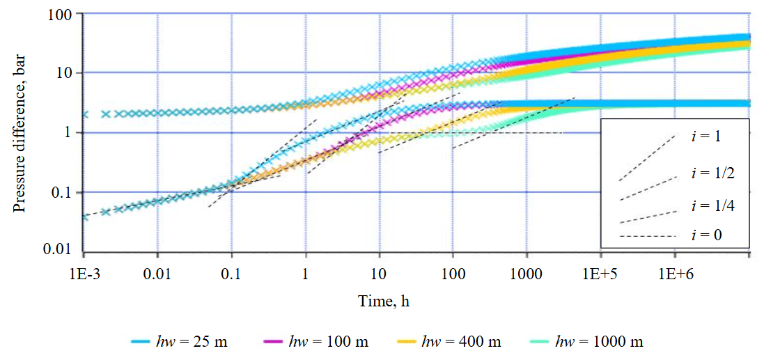
Fig.1. Demonstration of a pseudo-boundary-dominated flow case in a MFHW
Table 1
Parameters of MFHW
|
Parameter |
Value |
Parameter |
Value |
|
Permeability k, mD |
1 |
Initial pressure Pi, bar |
300 |
|
Porosity m, u.f. |
0.1 |
Number of fractures N |
3 |
|
Thickness h, m |
30 |
Fracture half-length Xf, m |
50 |
|
Total compressibility сt ·10–5, bar–1 |
3.6 |
Fracture conductivity Fc, mD·m |
300 |
|
Viscosity µ, mPa·s |
1 |
Liquid rate q, m3/day |
10 |
|
Formation volume factor B |
1 |
Skin factor S |
0.3 |
|
Well radius, mm |
99.4 |
|
|
Specifics of flow regimes manifestation for pressure buildup. The presence of a complex of flow regimes and regimes similar to those of a well operating in a bounded reservoir causes the behavior of the buildup in a MFHW to depend on the duration of its production before shut-in. Such processes are also observed during well testing in areas with unconfined reservoir boundaries. In the case of a short production period prior to shut-in, the subsequent buildup derivative exhibits a behavior in the early boundary response period that differs from the drawdown derivative. This behavior is caused by the peculiarities of the pressure response superposition related to the sealing boundary that occurred during production and subsequent shut-in [24, 26]. The pressure derivatives for the examples presented in Fig.1 exhibit similar behavior, with the most significant “distortion” observed in the cases demonstrating the pseudo-boundary-dominated flow. The change in behavior occurs within a specific range of the production duration Tpr, which depends on the given set of reservoir – well system parameters.
Such features of the derivative behavior are characterized by an interesting phenomenon that occurs for values of Tpr from the specific interval, where a difference in the shape of the buildup derivative compared to the drawdown derivative is observed. Figure 2 shows a comparison of the buildup and drawdown derivatives for the hw cases presented earlier; the buildup derivatives are plotted for different values of Tpr and hw. For all four hw cases, the buildup derivative shows the formation of a horizontal segment followed by a slight dip. Notably, a proximity is observed between the “plateau” of the early radial flow regime on the drawdown derivative and the developing “plateau” on the buildup derivative after a short flow period (Fig.2, d). It can be assumed that for the other cases as well, the appearance of a horizontal segment on the buildup after a short flow period may be a characteristic feature that allows for estimation of reservoir flow capacity without achieving the late radial flow regime.
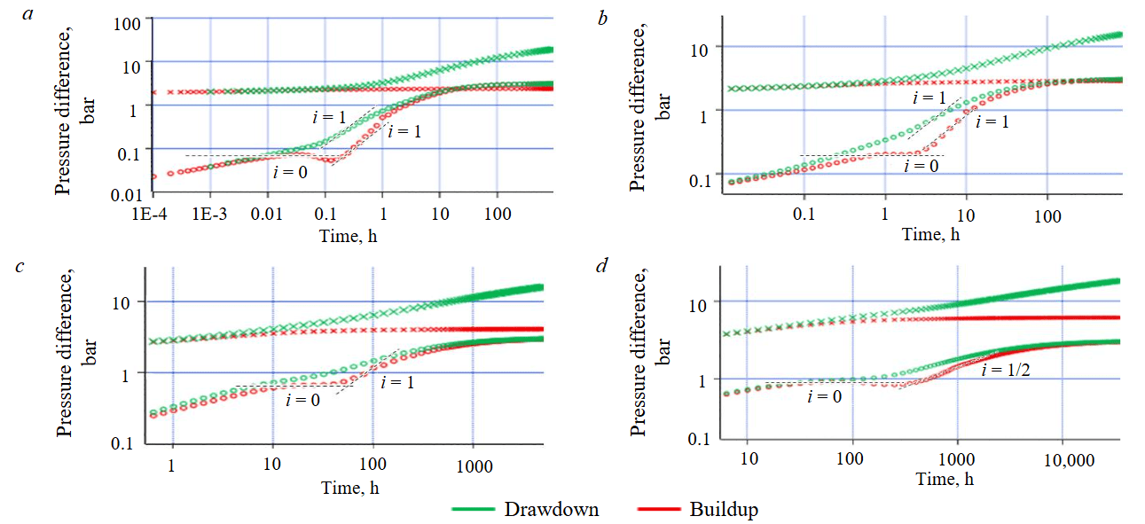
Fig.2. Close-up of the horizontal segment manifestation under a short-term production period conditions for various horizontal wellbore length scenarios: a – hw = 25 m, Tpr = 0.1 h; b – hw = 100 m, Tpr = 1 h; c – hw = 400 m, Tpr = 10 h; d – hw = 1000 m, Tpr = 100 h
Table 2 compares the values of the apparent permeability – thickness product (conductivity) khT, determined from the horizontal segment of the buildup derivative following a short flow period, with the initial (actual) reservoir – permeability thickness product khinit. The Table shows that the khT/khinit ratios do not exhibit a clear, unambiguous dependency. Only for the case of hw = 1000 m, which exhibits an early radial flow segment on the drawdown derivative, this ratio approaches the expected value – equal to the number of fractures N = 3 – though exceeding it by more than 10 %. In all other cases, the values are significantly higher, indicating a different flow regime that creates the “plateau” on the buildup derivative. Unlike the classic early radial flow regime, such a “plateau” also forms at low values of L/Xf, but specifically on the buildup derivative after a short flow period.
Table 2
Comparison of apparent conductivity with the initial value
|
hw,m |
khT, mD·m |
khinit, mD·m |
khT/khinit |
|
25 |
1283.7 |
30.0 |
42.8 |
|
100 |
459.4 |
30.0 |
15.3 |
|
400 |
140.3 |
30.0 |
4.7 |
|
1000 |
101.9 |
30.0 |
3.4 |
Dependence of the forming horizontal segment on the buildup derivative on the duration of transitional flow regimes. If the identified “plateau” on the buildup derivative is indeed related to the manifestation of a radial-flow-like regime, and not a result of overlapping transitional flow regimes, then its vertical position should not depend on parameters such as production time Tpr and system total compressibility ct. To analyze the influence of Tpr, a set of synthetic buildup curves was created for Tpr values ranging from 1 to 1000 h, using the reservoir – well system parameters presented in Table 3 (Fig.3, a). As can be seen, the buildup curves demonstrate the previously identified dependence of the derivative shape on the flowing time duration. And a distinct formation of a horizontal segment is observed at the same vertical level. Signs of the horizontal segment formation are observed at Tpr = 5 h and cease at Tpr = 500 h. It is worth noting the identical time for the start of the horizontal segment. A change in Tpr affects the duration of the horizontal segment's dominance.
Table 3
Parameters of MFHW for analyzing short-term production flow regime
|
Parameter |
Value |
Parameter |
Value |
|
Permeability k, mD |
1 |
Initial pressure Pi, bar |
112 |
|
Porosity m, u.f. |
0.25 |
Number of fractures N |
3 |
|
Thickness h, m |
25 |
Distance between the outermost fractures (length of the horizontal wellbore) hw, m |
450 |
|
Total compressibility сt ·10–5, bar–1 |
4.3 |
Fracture half-length Xf, m |
200 |
|
Viscosity µ, mPa·s |
1 |
Fracture conductivity Fc, mD·m |
500 |
|
Formation volume factor B |
1 |
Liquid rate q, m3/day |
10 |
|
Well radius, mm |
70 |
Skin factor S |
0.1 |
To assess the influence of system compressibility ct, the base case with parameters from Table 3 and production time Tpr of 100 h was used. The compressibility was varied when generating the synthetic curves until all signs of the horizontal segment manifestation disappeared. The range of values covered was 1∙10–6 to 3∙10–3 bar–1 (Fig.3, b). Similar to the production time variation, a change in compressibility does not affect the vertical position of the horizontal segment, the formation of which is observed at the same level. However, since variations in ct affect all temporal characteristics of the pressure buildup curves, not only the duration but also the time of the onset of the horizontal segment changes.
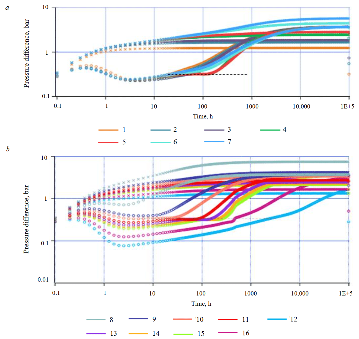
Fig.3. A family of pressure buildup curves for different values of Tpr (a) and ct (b)
1 – Tpr = 1 h; 2 – Tpr = 5 h; 3 – Tpr = 10 h; 4 – Tpr = 50 h; 5 – Tpr = 100 h; 6 – Tpr = 500 h; 7 – Tpr = 1000 h; 8 – ct = 1·10–6 bar–1; 9 – ct = 5·10–6 bar–1; 10 – ct = 1·10–5 bar–1; 11 – ct = 2.5·10–5 bar–1; 12 – ct = 3·10–3 bar–1; 13 – ct = 4.3·10–5 bar–1; 14 – ct = 6.5·10–5 bar–1; 15 – ct = 9·10–5 bar–1; 16 – ct = 5·10–4 bar–1
Thus, the identical vertical position of the horizontal segment on the buildup curves for different values of the flowing time Tpr and compressibility ct indicates that the formed “plateau” characterizes a specific radial-flow-like regime. The corresponding dependencies on reservoir and well parameters must be established for this regime.
Flow regime analysis from numerical simulation.To identify the characteristics of the flow regime associated with the emerging “plateau” on the derivative of the buildup after a short production period, let’s examine the dynamics of reservoir pressure distribution (drainage area formation) with numerical simulation. For this purpose, a simulation was performed using a 2D-numerical model in Kappa Saphir for the parameters of a MFHW presented in Table 3, with a production time of Tpr = 100 h. To identify potential differences in the buildup behavior, the simulation was conducted for fractures with both infinite and finite conductivity.
The diagnostic plot of the simulated buildup (Fig.4) reveals the following characteristic flow regimes:
- For the infinite conductivity fracture – linear flow with a derivative slope of i = 1/2, for the finite conductivity fracture – bilinear flow with i = 1/4 (at 1 h).
- A transitional flow regime (at 20 h).
- Early horizontal segment, i= 0 (60 h).
- A small dip in the derivative (120 h).
- Pseudo-boundary-dominated flow i= 1 (500 h).
- Late linear flow, i= 1/2 (2000 h).
- Late radial flow, i= 0 (6∙104 h).
As can be seen, with the exception of period 1, the presented segments of the buildup curves for the both fracture conductivity types are characterized by similar flow regimes. However, for the infinite conductivity fractures, the early horizontal segment on the derivative plot is positioned lower than for the finite conductivity fractures. Starting from the onset of the dominant pseudo-boundary-dominated flow (period 5), a convergence trend is observed in the pressure derivative curves, which become identical after the end of the late linear flow regime.
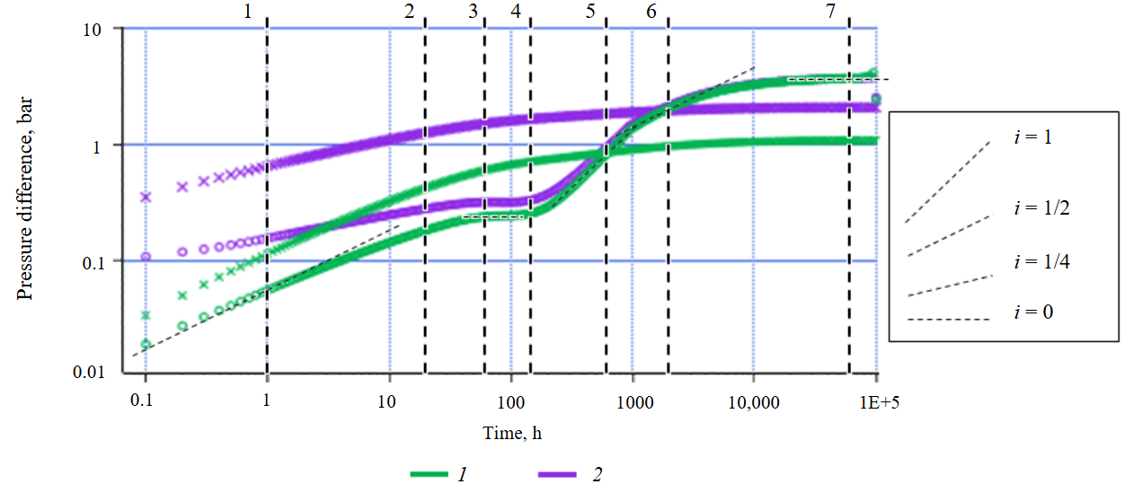
Fig.4. Diagnostic plot of a buildup for MFHW under a short-term production period conditions based on the data from Table 3
Infinite (1) and finite (2) conductivity fractures
In the case under consideration, following the bilinear flow regime for the finite conductivity fracture, an early linear flow regime does not develop. Instead, a transitional period and the formation of a horizontal segment are observed. The absence of linear flow is explained by the value of the dimensionless fracture conductivity CfD = Fc /(kXf ) = 2.5. It is known that for CfD values close to 1.6, the duration of the bilinear flow regime is maximized [26]. This accounts for the prolonged dominance of the bilinear flow regime in the presented example, which masks the linear flow segment preceding the formation of the early horizontal segment.
Figure 5 shows the pressure distributions around the wellbore, obtained from the pressure buildup simulation for infinite conductivity fractures, at the characteristic times marked by numbers in Fig.4:
- during the dominant linear flow period, the formation of low-pressure zones around the fractures is observed;
- during the transitional period, signs of weak interference between the fractures are noted;
- as the early horizontal segment forms, elliptical zones develop around the fractures;
- during the derivative dip, the ellipses around adjacent fractures merge (strong interference);
- the pseudo-boundary-dominated flow stage is characterized by the interference zones extending to the fracture tips;
- during the late linear (6) and radial (7) flow regimes, corresponding rectangular and circular drainage areas form around the horizontal wellbore.
Figure 6 presents similar pressure distributions for finite conductivity fractures. During the manifestation of the early horizontal segment 3, elliptical zones also form around the fractures, followed by their merging in the time interval corresponding to period 4. In the case of finite conductivity fractures the formed ellipses are more vertically compressed and only partially envelop the fracture surface. The reason for this is the development of low-pressure zones around the central part of the fractures during the dominant bilinear flow regime 1, which is caused by the pressure gradient inside the finite conductivity fracture. The subsequent development of the ellipse during stage 3 originates directly from the low-pressure zone formed during the dominant bilinear flow regime 1; therefore, its geometry is related to the fracture conductivity.
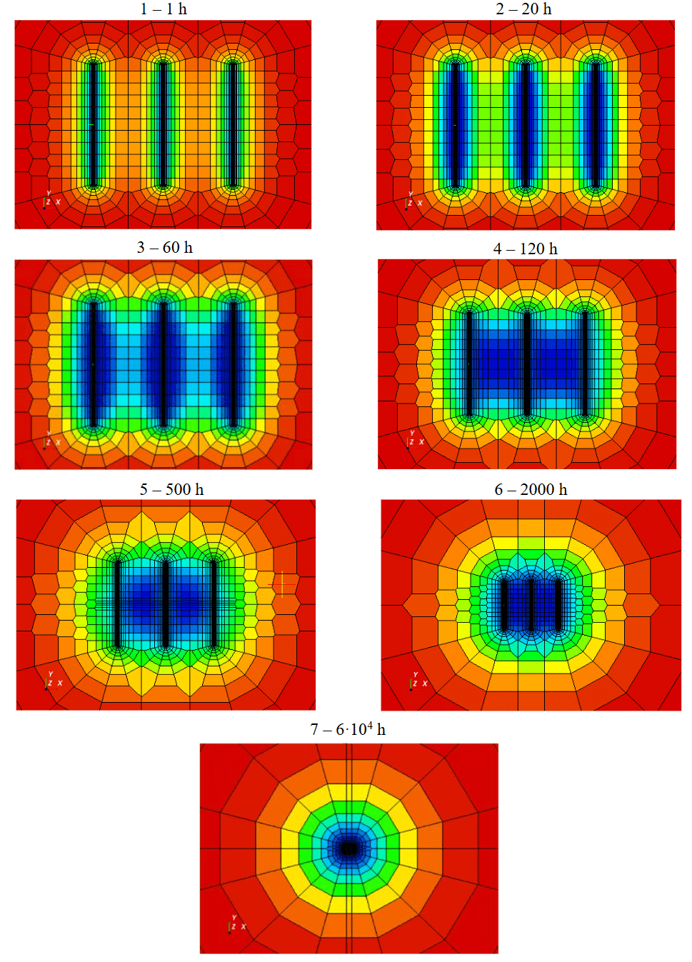
Fig.5. Pressure distributions at the times of dominant characteristic flow regimes. Infinite conductivity fractures
Blue corresponds to areas of minimum pressure, red – to maximum
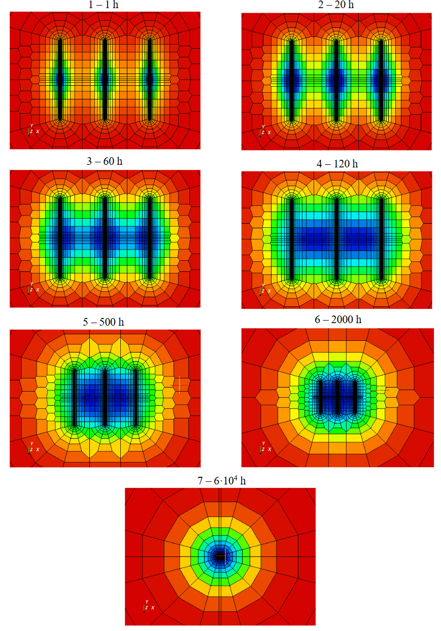
Fig.6. Pressure distributions at the times of dominant characteristic flow regimes. Finite conductivity fractures
For the legend, refer to Fig.5
Thus, the discrepancy in the pressure buildup behavior between the finite and infinite conductivity fracture models during periods 1-4 is due to the difference in the drained area. The subsequent time intervals are characterized by identical dynamics of drainage coverage. Overall, the presented numerical simulations lead to the conclusion that for MFHW, the manifestation of the early horizontal segment on the buildup after a short production period is associated with the development of a pseudo-radial (elliptical) flow regime around individual fractures. Due to the difference in the geometry of these areas from the strictly circular zones characteristic for the classical early radial flow regime, a different dependency between the position of the derivative “plateau” and the true reservoir flow capacity should be expected.
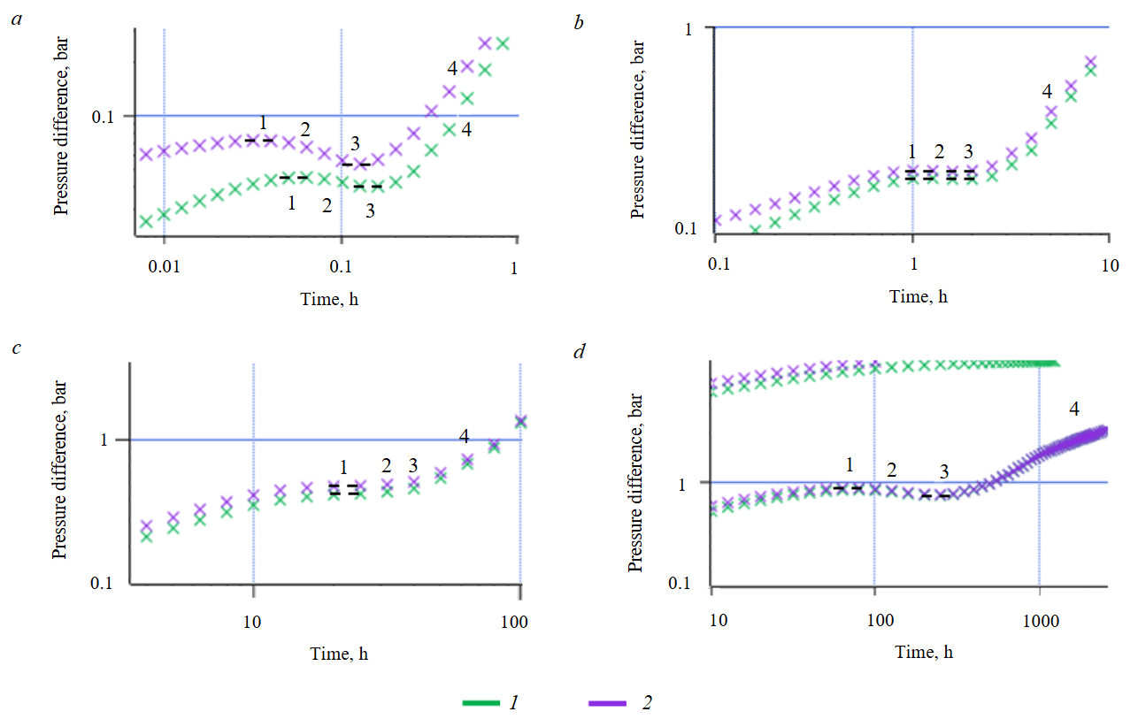
Fig.7. A comparison of diagnostic pressure buildup plots for infinite (1) and finite (2) conductivity fractures at the middle time period: a – hw = 25 m, Tpr = 0.1 h; b – hw = 100 m, Tpr = 1 h; c – hw = 400 m, Tpr = 10 h; d – hw = 1000 m, Tpr = 100 h
The difference in the behavior of the buildup derivative plots between the infinite and finite-conductivity fracture cases requires more detailed investigation. For this purpose, synthetic pressure buildup data were calculated for the two fracture conductivity types, using the previously considered values of horizontal wellbore lengths hw and the same reservoir – well system parameters (see Table 1).
Figure 7 compares the diagnostic plots of synthetic buildup data for infinite and finite conductivity fractures at the middle time period, for four values of hw. The numbers on the plot indicate the following characteristic flow regimes:
- Early horizontal segment.
- Derivative decline.
- Derivative minimum (“dip”).
- Pseudo-boundary-dominated flow.
For the most dense fracture spacing (Fig.7, a), the maximum discrepancy is observed between the plots for the infinite and finite conductivity fractures. As in Fig.4, the derivative for the infinite conductivity fractures runs lower. A discrepancy is also noted in the timing of flow regime manifestations: segment 1 (the early horizontal segment) appears later for the infinite conductivity fractures. As the distance between the outermost fractures (hw) increases in the other cases, a visual convergence of the curves is observed. However, in absolute terms, the difference in the position of the derivative “plateau” (segment 1) remains within one order of magnitude, in the range of 0.0175-0.046 bar (Table 4). At the same time, the time intervals of flow regime dominance are observed to be almost identical.
The evolving character of the derivative “dip” for different hw values is of particular interest. It has maximum for hw = 25 m, for hw = 100 m, a unified plateau forms during periods 1-3, for hw = 400 m, a slight increase in the derivative occurs in periods 2-3, while for hw = 1000 m, a decline in the derivative and its minimum are observed again.
Table 4
Comparison of the derivative “plateau” of horizontal segment 1 position for infinite and finite conductivity fractures
|
Fracture conductivity |
Position of horizontal segment |
|||||||
|
hw = 25 m |
hw = 100 m |
hw = 400 m |
hw = 1000 m |
|||||
|
i, bar |
Δ, bar |
i, bar |
Δ, bar |
i, bar |
Δ, bar |
i, bar |
Δ, bar |
|
|
Infinite |
0.0452 |
0.0277 |
0.186 |
0.0175 |
0.626 |
0.046 |
0.896 |
0.022 |
|
Finite |
0.0729 |
0.2035 |
0.672 |
0.918 |
||||
Table 5 summarizes the time values t for the midpoints of the four considered periods. Based on these values, the apparent investigation radii Rinv were determined using the corresponding option in Kappa Saphir. The radii are calculated according to the well-known relation involving the reservoir diffusivity coefficient [24, 27]. It should be noted that while the constant in the formula for Rinv can be chosen in different ways [28, 29], Kappa Saphir uses the most widespread expression, first substantiated by van Poolen in 1964 [24]. With the exception of the case with hw = 25 m, as well as segment 1 for the case with hw = 100 m, the times of the characteristic periods for finite and infinite conductivity fractures show no difference. The following patterns are identified:
- the period of the early horizontal segment on the buildup derivative corresponds to the time when the drained area has a horizontal dimension smaller than half the distance between the fractures L/2;
- as the drainage area expands and its horizontal dimension approaches L/2, interference processes between the fractures begin, causing the derivative to decline;
- at the derivative minimum (“dip”), the investigation radius (drainage area) is approximately equal to half the distance between the fractures Rinv ≈ L/2;
- during the pseudo-boundary-dominated flow period, the Rinv exceeds L/2 by approximately a factor of 1.5 to 2.
Table 5
Average time and investigation radius values for the four segments in case of infinite or finite conductivity fractures
|
Fracture conductivity |
The midpoint of the flow regime dominance interval |
|||||||
|
Section 1 |
Section 2 |
Section 3 |
Section 4 |
|||||
|
t, h |
Rinv, m |
t, h |
Rinv, m |
t, h |
Rinv, m |
t, h |
Rinv, m |
|
|
hw = 25 m (L/2 = 6.25 m) |
||||||||
|
Infinite |
0.0634 |
4.5 |
0.1005 |
5.6 |
0.159 |
7.1 |
0.5036 |
12.6 |
|
Finite |
0.0320 |
3.2 |
0.0798 |
5.0 |
0.127 |
6.3 |
0.318 |
10.0 |
|
hw = 100 m (L/2 = 25 m) |
||||||||
|
Infinite |
1.265 |
19.9 |
1.592 |
22.4 |
2.0475 |
25.4 |
5.0357 |
39.8 |
|
Finite |
1.0475 |
18.1 |
1.592 |
22.4 |
2.0475 |
25.4 |
5.0357 |
39.8 |
|
hw = 400 m (L/2 = 100 m) |
||||||||
|
Infinite |
20.0 |
79.4 |
25.2 |
89.0 |
40.0 |
112.1 |
79.8 |
158.3 |
|
Finite |
20.0 |
79.4 |
25.2 |
89.0 |
40.0 |
112.1 |
79.8 |
158.3 |
|
hw = 1000 m (L/2 = 250 m) |
||||||||
|
Infinite |
79.8 |
158.3 |
159.2 |
223.7 |
250.5 |
280.5 |
600.5 |
434.3 |
|
Finite |
79.8 |
158.3 |
159.2 |
223.7 |
250.5 |
280.5 |
600.5 |
434.3 |
The identified patterns are confirmed by analyzing the pressure distributions for the simulated cases over the considered time intervals. The corresponding plots are analogous to those in Fig.5 and 6 and are omitted for brevity. A clear correlation with the estimated investigation radius Rinv is observed in all cases without exception:
- during the manifestation of the horizontal segment on the pressure buildup derivative, ellipses form in the zone closest to the fractures;
- the derivative decline period is characterized by the coalescence of the ellipses between the fractures;
- at the moment of the derivative minimum (“dip”), a single region of reduced pressure forms within the space bounded by adjacent fractures;
- during the pseudo-boundary-dominated flow period, this region expands predominantly in the direction parallel to the fractures.
From these conclusions, the reasons for the most significant difference in pressure derivative behavior between the cases of infinite and finite conductivity fractures at hw = 25 m also become clear. They are caused by the most significant discrepancies in the geometry of the corresponding ellipses due to the most elongated shape of the regions between the fractures. For hw = 25 m, the differences in ellipse geometry are observed throughout the entire middle stage and are expected to disappear only when the drainage area extends beyond the fractures during the late linear flow regime. Furthermore, in this case with finite conductivity fractures, the drainage area in the space between the fractures is significantly smaller during all four flow regimes. This is what causes the higher position of the derivative “plateau” compared to the case of infinite conductivity fractures. For hw = 100 m, the differences are not as substantial, especially in flow regimes 3 and 4. This determines the proximity of the pressure derivatives between the two fracture conductivity cases. For hw = 400 m and hw = 1000 m, no visual differences are observed.
According to the visual assessment, the absence of a derivative “dip” for hw = 100 m is explained by the fact that even after the ellipses merge during flow regimes 2 and 3, the structure of elliptical flow is maintained for the both conductivity cases. Similarly, the onset of derivative growth from flow regime 2 for hw = 400 m is explained as follows: from the moment the ellipses merge, the drainage area begins to form a structure that is visually indistinguishable from the one formed during flow regime 4. For the cases of hw = 25 m and hw = 1000 m, each of the noted stages is characterized by the formation of a flow structure that differs from the previous one.
Thus, the results of numerical simulations demonstrate that the appearance of an early horizontal section on the pressure derivative plot, for a buildup following a short production period, is associated with the development of an elliptical flow regime around the hydraulic fractures. At the same time, the differences are observed in the geometric parameters of the resulting ellipses, which are determined by the fracture conductivity and fracture density. These differences, in turn, influence the vertical position of the derivative “plateau”.
Discussion
Analysis of the possibility to estimate reservoir properties from the biradial flow regime. In common well test interpretation practice and theory, the term “pseudo-radial flow regime” is used to describe the flow behavior at a radial-like flow regime characteristic at certain time periods for wells with a horizontal completion or a vertical hydraulic fracture [24, 30, 31]. It is considered that the pseudo-radial flow regime is entirely identical to the “conventional” radial flow regime in its diagnostic features. These features include a horizontal segment on the log-log pressure derivative plot and the methodology for estimating reservoir flow properties based on its vertical position. Thus, during a pseudo-radial flow regime, the lines of constant pressure are circles (and the drainage area is circular), considering coordinate axes scaling in the case of anisotropy.
However, a number of authors identify another characteristic radial-like type of flow, which typically occurs as a transitional regime between linear and pseudo-radial flow. It can be associated with the aforementioned completion types: vertically fractured wells [32-34], MFHW [35-37], and horizontal wells in naturally fractured reservoirs [38, 39]. The occurrence of this flow is also possible in the case of laterally anisotropic formations [32]. The shape of the constant-pressure lines (and the drainage area) at this regime is elliptical, and this term is sometimes applied to the regime itself. Depending on the underlying causes, the constant-pressure lines can be described either as similar ellipses with equivalent scaling towards a pseudo-radial configuration, or as confocal ellipses with a different flow geometry. Some publications use the synonymous term “biradial flow regime” for this behavior, a name that is apparently derived from the corresponding symmetry of the flow.
The diagnostic feature of the elliptical (biradial) flow regime was first described by D.Tiab in 1993 in his work [40]. Subsequently, other authors further developed the method he propo-sed [37, 41]. Based on a regression analysis of the curves that he constructed for an infinite conductivity fracture, D.Tiab derived the following equation for the pressure derivative with respect to time:
where Xe – half the length of the side of a closed rectangular area in which the flow is considered; tDA – the dimensionless time,
A – area; PD – dimensionless pressure,
In dimensional form, equation (1) becomes:
Here the product on the left side corresponds to the logarithmic derivative of the pressure change with respect to time (the Bourdet derivative). The area A is defined as the product of the lengths of the sides of the rectangular drainage area, 2Xe and 2Ye, where the direction of Xe is parallel to the fracture.
Let’s consider the applicability of D.Tiab's method to the elliptical flow identified above with the “plateau” on the buildup pressure derivative plot, which appears after a short production period. Based on Figures 5 and 6 and the estimates of the characteristic flow regime durations, assume that the bounding elliptical drainage zone develops within the fracture propagation area and half the distance between the adjacent fractures. Therefore, Xe = Xf, Ye = L/2.
From formula (2) proposed by D.Tiab, it is evident that during the period of the biradial flow dominance the logarithmic derivative plot should exhibit a straight-line segment with a slope of 0.36. Indeed, upon verification, the presence of such a regime is confirmed for the examples presented in Fig.7 for the both fracture conductivity cases.
Based on the presence of a characteristic diagnostic feature and the corresponding dependency, a preliminary estimate of reservoir flow capacity can be performed for the biradial flow regime, analogous to the early radial flow regime. According to formula (2), this estimate should be made by determining the value of the pressure derivative (tΔP′) at the time t corresponding to this regime:
For a MFHW, similarly to the early radial flow regime, it should be expected that the ratio of the obtained apparent flow capacity to the initial (actual) value should correspond to the number of fractures N. Note that the right side of expression (3) contains the diffusivity coefficient k/(mμct), which includes the permeability k. Therefore, estimating the flow capacity under real conditions requires a more complex calculation. However, to verify the method, it can be assumed that the diffusivity is a known quantity.
Table 6 presents the results of calculations for flow capacity using formula (3) for a section with a slope i = 0.36 for the cases shown in Fig.7. The last column shows the ratio of the resulting apparent flow capacity to the initial flow capacity. As can be seen from the table, the ratio value closest to the number of fractures N = 3 is observed for the case with hw = 25 m and a finite-conductivity fracture. However, this fact is more of a coincidence, since a general trend of decreasing the ratio with increasing fracture half-length is visible, and the values vary over a wide range. It is also evident that for hw = 25 m and hw = 100 m, a higher ratio value is characteristic of an infinite conductivity fracture.
Table 6
Comparison of the apparent (biradial) and initial (actual) flow capacity
|
Case |
Horizontal wellbore length hw, m |
Fc, mD·m |
(kh/μ)init, mD·m/mPa·s |
t, h |
tΔP′, bar |
(kh/μ)birad, mD·m/mPa·s |
(kh/μ)birad /(kh/μ)init |
|
1 |
25 |
Infinite |
30 |
0.005 |
0.0213 |
267.8 |
8.9 |
|
25 |
300 |
0.0556 |
102.6 |
3.4 |
|||
|
2 |
100 |
Infinite |
0.03 |
0.0553 |
62.6 |
2.1 |
|
|
100 |
300 |
0.0891 |
38.9 |
1.3 |
|||
|
3 |
400 |
Infinite |
4 |
0.479 |
48.7 |
1.6 |
|
|
400 |
300 |
||||||
|
4 |
1000 |
Infinite |
0.551 |
30.4 |
1.0 |
||
|
1000 |
300 |
Therefore, for the identified elliptical flow regime observed on the buildup pressure derivative for a MFHW after a short production period, the criteria for biradial flow with a derivative slope of i = 0.36 and the empirical formula by D.Tiab are not applicable. Further work should focus on analyzing the flow during the period when the derivative exhibits a horizontal segment and on investigating the dependence of the “plateau” position on the parameters of the reservoir – well system.
An empirical formula for flow capacity estimation from the horizontal segment of the elliptical flow regime.From the analysis presented above, the following conclusions can be drawn:
- the horizontal segment on the buildup derivative, following a short production period, corresponds to an elliptical flow regime;
- the position of the derivative “plateau” is expected to be related to both the reservoir flow properties (flow capacity) and the geometric characteristics of the elliptical flow formed in the reservoir – fracture system of MFHW.
To develop an expression for the position of the derivative “plateau”, 40 synthetic pressure buildup tests were simulated with variation of the following well – reservoir system parameters:
- Flow rate q.
- Permeability k.
- Pay zone h.
- Viscosity µ.
- Fracture half-length Xf.
- Length of the horizontal wellbore hw.
The parameters were selected based on their specific influences: some directly determine the “plateau” value of the horizontal segment during the late time (true) radial flow regime (q, k, h, µ), while others control the appearance of the horizontal segment and the geometry of the corresponding elliptical flow (Xf, hw). Parameter values were randomly sampled with the constraint that the buildup derivative must exhibit a horizontal segment corresponding to the elliptical flow regime after a production time of T = 100 h. At this stage of the study, only infinite conductivity fractures were considered to reduce the number of factors affecting the position of the horizontal segment.
Parameter values for each case and the corresponding calculation results are presented in Table 7. Column 12 provides flow capacity estimates from the segment with a slope of i = 0.36 for comparison. Despite the previously identified lack of correlation between the true flow capacity, the calculated value from the i = 0.36 segment, and the number of fractures, the current estimates by formula (3) accounted for the number of fractures based on theoretical considerations, analogous to the early radial flow regime:
Table 7
Initial parameters and flow capacity evaluation results for synthetic cases
|
Case |
q, m3/day |
k, mD |
h, m |
µ, mPa·s |
(kh/μ)init, mD·m/mPа·s |
Xf, m |
Length of horizontal wellbore hw, m |
Number of fractures N |
Distance between fractures L, m |
Section i = 0.36 (4) |
Section i = 0 (5) |
||||
|
tΔP′ at t = 1 h, bar |
kh/μ, mD·m/mPa·s |
δ, % |
tΔР′, bar |
kh/μ, mD·m/mPa·s |
δ, % |
||||||||||
|
1 |
2 |
3 |
4 |
5 |
6 |
7 |
8 |
9 |
10 |
11 |
12 |
13 |
14 |
15 |
16 |
|
1 |
10 |
0.7 |
15 |
6 |
1.8 |
100 |
1000 |
7 |
167 |
0.615 |
1.2 |
–33 |
2.143 |
1.8 |
3 |
|
2 |
20 |
0.7 |
23 |
15 |
1.1 |
60 |
300 |
5 |
75 |
1.267 |
3.0 |
182 |
7.818 |
1.0 |
–3 |
|
3 |
5 |
1 |
10 |
30 |
0.3 |
150 |
1000 |
10 |
111 |
1.520 |
0.2 |
–48 |
1.754 |
0.3 |
3 |
|
4 |
11 |
1 |
20 |
1 |
20.0 |
70 |
400 |
3 |
200 |
0.224 |
31.5 |
57 |
0.836 |
20.4 |
2 |
|
5 |
17 |
0.3 |
10 |
1 |
3.0 |
100 |
800 |
8 |
114 |
0.349 |
8.2 |
172 |
1.308 |
3.0 |
1 |
|
6 |
8 |
0.4 |
5 |
3 |
0.7 |
80 |
1200 |
9 |
150 |
0.520 |
1.7 |
152 |
4.050 |
0.7 |
1 |
|
7 |
26 |
2 |
30 |
25 |
2.4 |
130 |
300 |
4 |
100 |
0.477 |
10.8 |
352 |
3.485 |
2.3 |
–3 |
|
8 |
6 |
0.8 |
23 |
12 |
1.5 |
60 |
700 |
7 |
117 |
0.543 |
1.5 |
–4 |
1.712 |
1.6 |
3 |
|
9 |
14 |
0.8 |
14 |
3 |
3.7 |
80 |
200 |
3 |
100 |
0.672 |
10.2 |
172 |
2.687 |
3.5 |
–5 |
|
10 |
18 |
0.2 |
22 |
14 |
0.3 |
130 |
500 |
8 |
71 |
0.575 |
1.9 |
501 |
5.959 |
0.3 |
7 |
|
11 |
16 |
1.3 |
18 |
7 |
3.3 |
120 |
1000 |
10 |
111 |
0.151 |
11.3 |
239 |
0.702 |
3.4 |
3 |
|
12 |
27 |
1.7 |
24 |
5 |
8.2 |
120 |
550 |
4 |
183 |
0.324 |
23.1 |
183 |
2.056 |
8.2 |
0 |
|
13 |
8 |
0.9 |
26 |
9 |
2.6 |
150 |
200 |
3 |
100 |
0.202 |
10.8 |
315 |
1.153 |
2.5 |
–3 |
|
14 |
13 |
0.7 |
19 |
13 |
1.0 |
120 |
900 |
9 |
113 |
0.266 |
3.7 |
261 |
2.085 |
1.1 |
3 |
|
15 |
21 |
1.7 |
17 |
9 |
3.2 |
70 |
1100 |
10 |
122 |
0.358 |
7.4 |
130 |
1.784 |
3.3 |
4 |
|
16 |
19 |
2 |
10 |
18 |
1.1 |
80 |
500 |
5 |
125 |
1.297 |
2.9 |
159 |
8.586 |
1.1 |
1 |
|
17 |
17 |
0.7 |
16 |
4 |
2.8 |
120 |
400 |
4 |
133 |
0.489 |
8.5 |
203 |
2.774 |
2.8 |
–1 |
|
18 |
15 |
1.1 |
19 |
11 |
1.9 |
60 |
800 |
9 |
100 |
0.392 |
4.8 |
155 |
2.303 |
2.0 |
3 |
|
19 |
13 |
1.7 |
23 |
6 |
6.5 |
130 |
400 |
5 |
100 |
0.128 |
25.6 |
292 |
0.485 |
6.7 |
3 |
|
20 |
24 |
1.3 |
35 |
23 |
2.0 |
100 |
1000 |
9 |
125 |
0.285 |
6.7 |
237 |
2.612 |
2.1 |
5 |
|
21 |
70 |
2 |
21 |
8 |
5.3 |
70 |
700 |
4 |
233 |
2.025 |
9.5 |
82 |
16.399 |
5.8 |
10 |
|
22 |
15 |
1 |
6 |
16 |
0.4 |
97 |
800 |
7 |
133 |
1.365 |
1.1 |
205 |
12.211 |
0.4 |
5 |
|
23 |
15 |
0.5 |
18 |
25 |
0.4 |
108 |
700 |
8 |
100 |
0.605 |
1.6 |
345 |
7.034 |
0.4 |
12 |
|
24 |
55 |
1.3 |
10 |
7 |
1.9 |
119 |
500 |
7 |
83 |
1.290 |
7.2 |
289 |
4.566 |
2.0 |
6 |
|
25 |
10 |
1.2 |
12 |
10 |
1.4 |
98 |
700 |
7 |
117 |
0.304 |
4.5 |
215 |
1.891 |
1.5 |
2 |
|
26 |
29 |
0.3 |
18 |
11 |
0.5 |
75 |
500 |
9 |
63 |
1.197 |
2.1 |
327 |
8.797 |
0.5 |
1 |
|
27 |
45 |
1.5 |
34 |
8 |
6.4 |
140 |
500 |
3 |
250 |
0.649 |
17.5 |
174 |
6.609 |
6.6 |
4 |
|
28 |
53 |
0.7 |
26 |
11 |
1.7 |
132 |
700 |
10 |
78 |
0.541 |
7.8 |
372 |
2.982 |
1.7 |
3 |
|
29 |
15 |
1.7 |
6 |
21 |
0.5 |
130 |
900 |
9 |
113 |
0.668 |
1.9 |
293 |
4.775 |
0.5 |
1 |
|
30 |
9 |
0.8 |
24 |
15 |
1.3 |
141 |
600 |
5 |
150 |
0.209 |
5.0 |
289 |
2.270 |
1.4 |
7 |
|
31 |
12 |
0.6 |
14 |
24 |
0.4 |
87 |
500 |
9 |
63 |
0.617 |
1.5 |
342 |
4.409 |
0.4 |
1 |
|
32 |
32 |
1.5 |
16 |
23 |
1.0 |
137 |
1200 |
8 |
171 |
0.584 |
4.1 |
292 |
7.217 |
1.1 |
8 |
|
33 |
67 |
1 |
25 |
8 |
3.1 |
98 |
500 |
5 |
125 |
1.399 |
9.1 |
192 |
8.855 |
3.1 |
1 |
|
34 |
12 |
1.6 |
8 |
27 |
0.5 |
120 |
900 |
6 |
180 |
0.752 |
1.6 |
234 |
9.332 |
0.5 |
10 |
|
35 |
60 |
1.1 |
24 |
1 |
26.4 |
145 |
1200 |
6 |
240 |
0.226 |
63.3 |
140 |
0.988 |
27.3 |
3 |
|
36 |
37 |
0.8 |
33 |
26 |
1.0 |
69 |
1000 |
9 |
125 |
0.926 |
2.9 |
186 |
10.706 |
1.1 |
12 |
|
37 |
18 |
0.7 |
11 |
22 |
0.4 |
91 |
500 |
5 |
125 |
1.959 |
1.1 |
214 |
21.820 |
0.4 |
5 |
|
38 |
54 |
1.9 |
19 |
28 |
1.3 |
132 |
1100 |
7 |
183 |
1.070 |
4.3 |
235 |
12.250 |
1.4 |
10 |
|
39 |
14 |
1.7 |
26 |
23 |
1.9 |
145 |
800 |
7 |
133 |
0.194 |
6.9 |
260 |
1.514 |
2.0 |
3 |
|
40 |
8 |
1.5 |
15 |
4 |
5.6 |
148 |
1000 |
6 |
200 |
0.081 |
17.0 |
201 |
0.514 |
5.7 |
1 |
As can be seen from column 13, an acceptable percentage error in flow capacity estimation using formula (4) (4 %) is observed only for case 8. Overall, the mean absolute percentage error across all cases is δ = 218 %, which further confirms the irrelevance of estimating reservoir parameters from the derivative segment with a slope of i = 0.36.
An empirical expression was developed for estimating flow capacity from the “plateau” of the elliptical flow regime horizontal segment, based on the following considerations. For a classical radial flow regime, the contribution of the axisymmetric flow geometry to the relationship between the flow rate and flow capacity is determined by the wellbore boundary condition, which is derived from Darcyʼs law:
where h2πr corresponds to the wellbore wall area (with 2πr being its perimeter), through which inflow occurs; and is the pressure gradient.
The well is approximated as a line source with a radius rw → 0. This results in the final solution including only a factor of 2π as the complex contribution of the wellbore wall perimeter and the distance affecting the acting pressure gradient.
In the case of elliptical flow to an infinite conductivity fracture, the source is represented by the fracture surface with a non-zero perimeter of 4Xf (and an area of 4Xfh). The pressure gradient must be related to half the distance between the fractures, L/2. By incorporating both of these quantities into the relevant parts of the formula for the position of the derivative “plateau” and adjusting the missing multiplier, the following empirical relationship was identified:
or
The results of the flow capacity estimation based on the “plateau” of the horizontal section of the elliptical flow regime, using formula (5), are presented in column 15 of Table 7. The corresponding error values are provided in column 16. The error in estimating the flow capacity does not exceed 12 % and, for the majority of cases, remains within the 5-6 % range, with an average value of 4.05 %.
By denoting the left side of formula (6) as PD, the accuracy of the obtained empirical relationship can be further assessed by comparing its value to 1 for all cases considered. According to the evaluation results, the average PD value across the cases differs from 1 but is characterized by a close value of 0.969. Furthermore, in none of the cases does the error exceed the 15 % threshold, which is considered critical from the standpoint of common well test interpretation practice.
Therefore, although the empirical relationship (5) introduces a slight bias in the estimates for the dataset considered, the obtained results indicate its practical applicability, unlike the estimates from the section with a slope of i = 0.36. It should be noted that, based on the nature of the pressure distributions in Figures 5 and 6, relationship (5) can potentially be generalized to the case of finite-conductivity fractures. This would require replacing the quantity Xf with the equivalent length of the region inside the fracture affected by pressure redistribution by the time the elliptical flow regime develops.
Despite the obtained optimistic results, the range of applicability of the empirical formula (5) requires further investigation. For sufficiently large distances between fractures, the elliptical flow regime “plateau” on the buildup derivative begins to coincide with the emerging early radial flow regime “plateau” on the drawdown derivative. Consequently, formula (5) must transition into the classical flow capacity estimation formula for the radial flow regime, adjusted for the number of fractures.
Specifically, the distance between fractures for the cases in Table 7 ranges from 63 to 250 m, with an average value of 132 m. It is of interest to test cases outside this range. For this purpose, let’s return to the four previously considered scenarios with horizontal wellbore lengths hw of 25, 100, 400 and 1000 m for N = 3. The corresponding PD values for these are 0.994, 1.023, 0.865 and 0.493, respectively. As can be seen, for the cases with hw = 25 m and hw = 100 m, whose L values (12.5 and 50 m, respectively) are below the minimum value of the aforementioned range, the PD value is even closer to unity than in most of the previously considered cases. For hw = 400 m (L = 200 m), the deviation of PD from unity is significantly higher but still falls within the 15 % threshold. A substantial deviation (over 50 %) is observed only for the case with hw = 1000 m (L = = 500 m), which exhibits a clearly defined early radial flow regime on the drawdown derivative. This confirms the conclusion that the relationship (5) for infinite conductivity fractures ceases to be valid when the distance between the fractures is significantly increased relative to their half-length Xf.
Practical applications of the elliptical flow regime. Given that the emergence of the elliptical flow regime requires a short production period, the most practical scenario for its observation is the testing of new wells that are put into production directly after drilling. Such a test requires a short cleanup period, which should be followed by a pressure buildup test. The necessary durations of both the production and shut-in periods must be determined through well test design, which involves generating synthetic derivative curves based on the well configuration (number of fractures and spacing) and expected reservoir – well system parameters. This test design includes a sensitivity analysis to account for input data uncertainty. Upon completion of the buildup, the well is put back into production. This may be for further cleanup, for productivity (inflow performance relationship) testing, or to begin regular production to the gathering line.
Another practical application scenario involves wells that have been returned to service after an extended shutdown due to various operational reasons. In this case, a well test design must also be developed. The design is used to assess both the feasibility of obtaining an elliptical flow regime (i.e., the sufficiency of the shut-in time) and the necessary durations for the production period and the subsequent buildup.
Conclusion
Reliable assessment of the well – reservoir system parameters from the interpretation of well test data of MFHW in low-permeability reservoirs is associated with significant difficulties. This is due to the practically unattainable time required to reach the late radial flow regime and, consequently, the high uncertainty in estimating the reservoir flow capacity. An alternative solution is to estimate the flow capacity using data from the early radial flow regime. However, the corresponding horizontal segment appears on the pressure derivative log-log plot only when the distances between fractures are sufficiently large compared to their half-length.
The analytical and numerical calculations presented and analyzed in this paper for a significant number of synthetic cases demonstrate that with a sufficiently short production period before the well shut-in, a different type of radial-like flow regime can appear in a pressure buildup test. This regime is also characterized by the formation of a horizontal “plateau” on the derivative plot, potentially followed by a “dip” and a transition to the pseudo-boundary-dominated flow regime in the region between fractures, indicated by a unit slope on the derivative plot. The identified radial-like flow regime is characterized by an elliptical shape of the drainage zones in the region between the fractures and ceases when these zones close up due to the onset of strong fracture interference. The vertical position of the derivative “plateau” is stable with respect to the producing time and the total system compressibility and is related to the reservoir flow capacity and fracture parameters (number of fractures, their half-length, conductivity and spacing).
Application of the D.Tiab’s empirical method, which relies on a derivative segment with a slope of 0.36 (biradial flow regime), to the identified elliptical flow regime leads to significant errors (off by a factor of several times) in the estimation of flow capacity and has no practical potential. Given the observed geometry of the developed elliptical flow, an empirical formula has been proposed to estimate the flow capacity based on the derivative “plateau” for the case of infinite-conductivity fractures. The formula has demonstrated sufficient accuracy for practical application (error no greater than 12 %, average of about 4 %) for relatively small fracture spacings. The estimation accuracy decreases as the spacing between fractures increases.
The results of this study enable more informative well tests of MFHW in low-permeability reservoirs, enabling reliable assessment of the well – reservoir system parameters. This is achieved through a combination of a short production period, for instance after drilling, and a subsequent shut-in for a pressure buildup test. The effective design of such tests, depending on specific reservoir features and well completion design, is the subject of further research.
Further investigation is required to determine the applicability domain of the proposed empirical formula and/or its refinement. This is necessary for accurately estimating flow capacity during the transition from the identified elliptical flow regime to the known early radial flow regime at larger fracture spacings. Additionally, generalizing the formula to account for finite conductivity fractures is also of significant practical interest.
References
- Arzhilovsky A.V., Grischenko A.S., Smirnov D.S. A case study of drilling horizontal wells with multistage hy-draulic fracturing in low-permeable reservoirs of the Tyumen formation at the fields of RN-Uvatneftegas. Oil Indus-try Journal. 2021. N 2, p. 74-76 (in Russian). DOI: 10.24887/0028-2448-2021-2-74-76
- Walker L. Technology Focus: Unconventional and Tight Reservoirs (July 2024). Journal of Petroleum Technology. 2024. Vol. 76. Iss. 7, p. 88-89. DOI: 10.2118/0724-0088-JPT
- Manuaba I.B.G.H., Aljishi M., Van Steene M., Dolan J. Logging-While-Drilling Laterolog vs. Electromagnetic Propagation Measurements: Which Is Telling the True Resistivity? SPE Journal. 2024. Vol. 29. Iss. 8, p. 4000-4013. DOI: 10.2118/219772-PA
- Carpenter C. Holistic Approach Uses Electromagnetic Tools, LWD Data To Improve Reservoir Understanding. Journal of Petroleum Technology. 2024. Vol. 76. Iss. 1, p. 95-97. DOI: 10.2118/0124-0095-JPT
- Belova A.A., Ovchinnikov K.N., Buyanov A.V. et al. Long-term monitoring of gas flow to a horizontal well after multistage hydraulic fracturing using tracer polymer technologies. Gas Industry Journal. 2020. N 9 (806), p. 86-94 (in Russian).
- Asmandiyarov R.N., Ipatov A.I., Yazkov A.V. et al. Gazprom Neft’s experience in testing commercial marker monitoring systems for oil wells and in assessing their reliability. Oil Industry Journal. 2023. N 12, p. 53-57 (in Russian). DOI: 10.24887/0028-2448-2023-12-53-57
- Zhenzhen Wang, Chen Li, King M.J. Applications of Asymptotic Solutions of the Diffusivity Equation to Infinite Acting Pressure Transient Analysis. SPE Journal. 2024. Vol. 29. Iss. 8, p. 4069-4093. DOI: 10.2118/180149-PA
- Kremenetskii M.I., Ipatov A.I. Application of production logging to optimize oil and gas field development. In 2 vol. Vol. 1. Fundamentals of well testing and production logging control of field development and production monitoring. Moscow; Izhevsk: IKI, 2020, p. 660 (in Russian).
- Ipatov A.I., Kremenetsky M.I. Problems of field development control in the context of the “new economic policy”. Actual Problems of Oil and Gas. 2022. Iss. 2 (37), p. 87-99 (in Russian). DOI: 10.29222/ipng.2078-5712.2022-37.art6
- Grishina E.I., Kremenetsky M.I., Buyanov A.V. Forecast of a heterogeneous formation in horizontal wells subjected to a multistage hydraulic fracturing by the data of integrated geophysical and hydrodynamic studies. Oilfield Engineering. 2020. N 5 (617), p. 38-43 (in Russian). DOI: 10.30713/0207-2351-2020-5(617)-38-43
- Ipatov A.I., Kremenetskiy M.I., Gulyaev D.N. et al. Reservoir surveillance when hard-to-recover reserves developing. Oil Industry Journal. 2015. N 9, p. 68-72 (in Russian).
- Grishina E. Using Well Testing and Production Logging Methods to Estimate Individual Frature's Parametres and Perfor-mance in a Fractured Horizontal. SPE Russian Petroleum Technology Conference, 15-17 October 2018, Moscow, Russia. OnePetro, 2018. N SPE-191563-18RPTC-MS. DOI: 10.2118/191563-18RPTC-MS
- Kremenetskiy M., Kokurina V., Morozovskiy N., Grishina E. PI Evaluation by Well Tests in Case of Low Permeability Formations Exposed by Complex Geometry Fracs. SPE Russian Petroleum Technology Conference, 16-18 October 2017, Moscow, Russia. OnePetro, 2017. N SPE-187766-MS. DOI: 10.2118/187766-MS
- Kovalenko I.V. Invariant of dependence between flux and capacitive parameters at transient flow to the wells with multi-stage hydraulic fracturing as an instrument of well test data interpretation. Oilfield Engineering. 2022. N 8 (644), p. 13-20 (in Russian). DOI: 10.33285/0207-2351-2022-8(644)-13-20
- Kovalenko I.V. Forecasting the productivity of horizontal wells with multistage hydraulic fracturing: Avtoref. dis. … d-ra tekhn. nauk. Tyumen: Tyumenskii industrialnyi universitet, 2021, p. 38 (in Russian).
- Nikonorova A.N., Voron K.A., Kremenetsky M.I. et al. Evaluation of production potential dynamics of oil and gas horizontal wells with multi-stage hydraulic fracturing based on early flow regimes at pressure transient analysis. Exposition Oil Gas. 2024. N 6 (107), p. 50-56 (in Russian). DOI: 10.24412/2076-6785-2024-6-50-56
- Tulenkov S.V., Tulenkova S.V., Mamonov D.M. et al. Testing deconvolution when interpreting flow test data from hydraulically-fractured wells in gas-saturated low-permeable achimov reservoirs. Scientific Journal of the Russian Gas Society. 2024. N 3 (45), p. 102-109 (in Russian).
- Asalkhuzina G.F., Davletbaev A.Ya., Abdullin R.I. et al. Welltesting for a linear development system in low permeability formation. Oil and Gas Fields Development. 2021. Vol. 19. N 3, p. 49-58 (in Russian). DOI: 10.17122/ngdelo-2021-3-49-58
- Martyushev D.A., Yongfei Yang, Kazemzadeh Y. et al. Understanding the Mechanism of Hydraulic Fracturing in Naturally Fractured Carbonate Reservoirs: Microseismic Monitoring and Well Testing. Arabian Journal for Science and Engineering. 2024. Vol. 49. Iss. 6, p. 8573-8586. DOI: 10.1007/s13369-023-08513-1
- Galkin V.I., Martyushev D.A., Ponomareva I.N., Chernykh I.A. Developing features of the near-bottomhole zones in productive formations at fields with high gas saturation of formation oil. Journal of Mining Institute. 2021. Vol. 249, p. 386-392. DOI: 10.31897/PMI.2021.3.7
- Salnikova O.L., Chernykh I.A., Martyushev D.A., Ponomareva I.N. Features of determining filtration parameters of complex carbonate reservoirs at their operation by horizontal wells. Bulletin of the Tomsk Polytechnic University. Geo Assets Engineering. 2023. Vol. 334. N 5, p. 138-147 (in Russian). DOI: 10.18799/24131830/2023/5/3970
- Grishina E.I. Production logging and well testing control of heterogeneous reservoir development based on invariant pa-rameters in wells with high-tech completions: Avtoref. dis. … kand. tekhn. nauk. Moscow: Rossiiskii gosudarstvennyi universitet nefti i gaza (natsionalnyi issledovatelskii universitet) imeni I.M.Gubkina, 2021, p. 24 (in Russian).
- Kremenetskii M.I., Ipatov A.I. Application of Field Geophysical Control to Optimize the Development of Oil and Gas Fields. In 2 vol. Vol. 2. The Role of Well Testing and Production Logging in Reservoir Development. Moscow; Izhevsk: IKI, 2020, p. 756 (in Russian).
- Houzé O., Viturat D., Fjaere O.S. et al. Dynamic Data Analysis, v5.42. Kappa, 1988-2021, p. 776.
- Wentao Zhou, Raj Banerjee, Poe B. et al. Semianalytical Production Simulation of Complex Hydraulic-Fracture Networks. SPE Journal. 2014. Vol. 19. Iss. 1, p. 6-18. DOI: 10.2118/157367-PA
- Transient Well Testing / Ed. by M.M.Kamal. Society of Petroleum Engineers, 2009, p. 860.
- Horne R.N. Modern Well Test Analysis: A Computer-Aided Approach. Petroway, 1995, p. 257.
- Hossain M.E., Tamim M., Rahman N.M.A. Effects of Criterion Values on Estimation of the Radius of Drainage and Stabi-lization Time. Journal of Canadian Petroleum Technology. 2007. Vol. 46. Iss. 3, p. 24-30. DOI: 10.2118/07-03-01
- Ramakrishnan T.S., Prange M.D., Kuchuk F.J. Radius of Investigation in Pressure Transient Testing. Transport in Porous Media. 2020. Vol. 131. Iss. 3, p. 783-804. DOI: 10.1007/s11242-019-01367-y
- Mazhar V.A., Ridel A.A., Kolesnikov M.V. et al. The practice of hydrodynamic surveys in complex design wells. Actual Problems of Oil and Gas. 2022. Iss. 2 (37), p. 127-138 (in Russian). DOI: 10.29222/ipng.2078-5712.2022-37.art9
- Sergeev V.L., Dong Van Hoang. Adaptive interpretation of pressure transient tests of horizontal wells with pseudoradial flow identification. Bulletin of the Tomsk Polytechnic University. Geo Аssets Engineering. 2017. Vol. 328. N 10, p. 67-73 (in Russian).
- Kuchuk F., Bringham W.E. Transient Flow in Elliptical Systems. Society of Petroleum Engineers Journal. 1979. Vol. 19. Iss. 6, p. 401-410. DOI: 10.2118/7488-PA
- Escobar F.-H., Montealegre M.M., Cantillo J.-H. Conventional analysis for characterization of bi-radial (elliptical) flow in infinite-conductivity vertical fractured wells. CT&F – Ciencia, Tecnología y Futuro. 2006. Vol. 3. N 2, p. 141-147.
- Amini S., Ilk D., Blasingame T.A. Evaluation of the Elliptical Flow Period for Hydraulically-Fractured Wells in Tight Gas Sands – Theoretical Aspects and Practical Considerations. SPE Hydraulic Fracturing Technology Conference, 29-31 January 2007, College Station, TX, USA. OnePetro, 2007. N SPE-106308-MS. DOI: 10.2118/106308-MS
- Badazhkov D., Ovsyannikov D., Kovalenko A. Analysis of Production Data with Elliptical Flow Regime in Tight Gas Reservoirs. SPE Russian Oil and Gas Technical Conference and Exhibition, 28-30 October 2008, Moscow, Russia. OnePetro, 2008. N SPE-117023-MS. DOI: 10.2118/117023-MS
- Weiyao Zhu, Yunfeng Liu, Zhongxing Li et al. Study on Pressure Propagation in Tight Oil Reservoirs with Stimulated Reservoir Volume Development. ACS Omega. 2021. Vol. 6. Iss. 4, p. 2589-2600. DOI: 10.1021/acsomega.0c04661
- Apte S.S., Lee W.J. Elliptical Flow Regimes in Horizontal Wells with Multiple Hydraulic Fractures. SPE Hydraulic Fracturing Technology Conference and Exhibition, 24-26 January 2017, the Woodlands, TX, USA. OnePetro, 2017. N SPE-184856-MS. DOI: 10.2118/184856-MS
- Escobar F.H., Ghisays-Ruiz A., Bonilla L.F. New model for elliptical flow regime in hydraulically-fractured vertical wells in homogeneous and naturally-fractured systems. ARPN Journal of Engineering and Applied Sciences. 2014. Vol. 9. N 9, p. 1629-1636.
- Zhiming Chen, Xinwei Liao, Wei Yu, Sepehrnoori K. Pressure-Transient Behaviors of Wells in Fractured Reservoirs With Natural- and Hydraulic-Fracture Networks. SPE Journal. 2019. Vol. 24. Iss. 1, p. 375-394. DOI: 10.2118/194013-PA
- Tiab D. Analysis of Pressure and Pressure Derivative without Type-Curve Matching – III. Vertically Fractured Wells in Closed Systems. SPE Western Regional Meeting, 26-28 May 1993, Anchorage, AK, USA. OnePetro, 1993. N SPE-26138-MS. DOI: 10.2118/26138-MS
- Malallah A., Nashawi I.S., Algharaib M. A comprehensive analysis of transient rate and rate derivative data of an oil well intercepted by infinite-conductivity hydraulic fracture in closed systems. Journal of Petroleum Exploration and Production Technology. 2024. Vol. 14. Iss. 3, p. 805-822. DOI: 10.1007/s13202-023-01732-0