
Interpretable machine learning to detect well integrity issues
- 1 — Engineer of the I Category Tatar Oil Research and Design Institute (TatNIPIneft) of PJSC TATNEFT ▪ Orcid ▪ Elibrary
- 2 — Ph.D., Dr.Sci. Director for Enhanced Oil Recovery, Wave Technology and Biotechnology Tatar Oil Research and Design Institute (TatNIPIneft) of PJSC TATNEFT ▪ Orcid
Abstract
The problem of timely and accurate evaluation of well integrity is becoming increasingly relevant in the context of mature field development, high wellstream water cut, and a growing number of old wells. For production casing diagnostics, geophysical methods are typically used to identify damage and determine its interval. However, high workload of field personnel hinders prompt deployment of wireline crews to survey the integrity of wells. This results in lost oil production, increased water cut, environmental risks, increased non-productive injected volumes, and reduced key economic indices. To address these challenges, a novel approach to evaluation of casing string integrity based on machine learning models has been proposed. The paper presents a procedure for application of interpretable machine learning to detect production casing leakage and provides a comparison of this approach with the ROC-AUC statistical analysis method. The novel approach integrates the LightGBM machine learning algorithm and SHAP analysis to evaluate contribution of key features to well integrity prediction and determine their threshold values. The model training was based on data from 14,318 well surveys conducted between 2000 and 2022. The results indicate that the most important features are sulfate content, solution supersaturation ratio, and water cut. The study confirms the efficiency of interpretable machine learning methods for diagnosing complex technical systems. These results show the potential for application of such models in well integrity monitoring and well workover planning. This approach can also be used in other oil and gas applications, such as prediction of various problems and optimization of well operation conditions.
None
Introduction
The problem of casing leakage is one of the most critical issues in oil field development. Loss of casing integrity results in oil production rate decrease, water cut increase, and significant environmental risks [1]. Conventional diagnostic methods for casing leakage typically involve well logging, water chemical analysis, and mathematical modeling [2-4]. However, all these methods have a number of disadvantages: high cost, complexity of data interpretation, and time-consuming studies [5, 6]. Magnetic pulsed inspection has limitations under high-temperature and high-pressure (HPHT) conditions, which reduces its efficiency in challenging downhole environment [5], while thermal convection monitoring requires precise calibration and specialized equipment, increasing diagnostic costs [6]. Consequently, there is a growing need in implementation of modern technologies for casing integrity monitoring, particularly machine learning methods which can enhance prediction accuracy and promptness of damage detection.
Geophysical surveys such as noise logging, temperature logging, and acoustic logging are the most common methods for detecting production casing leaks. For instance, tracer surveys enable efficient localization of behind-the-casing flow [7].
Produced water chemical analysis is an alternative, readily available diagnostic method. Changes in the concentration of chemical components, such as sulfates and chlorides, can indicate behind-the-casing flow and fluid inflow from other formations [8]. Water-oil ratio and well stream water cut analysis serve as important indicators of casing integrity failure [9, 10]. However, in case of complex geochemical sections, this method is less accurate than geophysical techniques.
Application of mathematical modeling makes it possible to forecast the development of behind-the-casing flow and optimize squeeze jobs. The paper [11] presents models considering the process dynamics during the waiting-on-cement period. The paper [12] proposes an innovative method for remedial cementing which minimizes economic risks and improves squeeze job efficiency. Thus, the combination of geophysical methods, chemical analysis, and mathematical modeling provides the basis for comprehensive diagnostics of production casing leakage. However, the limitations of conventional methods necessitate implementation of innovative approaches, such as machine learning. Machine learning methods make it possible to analyze large datasets, account for non-linear relationships, and enhance the accuracy of development parameter forecasting [11-14]. They are frequently used for predicting oil production rates, reservoir pressure, and other parameters. The paper [11] presents a procedure for predicting oil properties in situ using neural networks. The authors of paper [14] improved conventional decline curve analysis methods by applying Random Forest and Gradient Boosting algorithms, which allowed increasing the accuracy of forecasts. The paper [15] proposes a method for intake pressure recovery in wells equipped with electrical submersible pumps based on the analysis of water cut and other parameters.
The paper [16] discusses a multi-target regression based on the Random Forest algorithm to predict shale gas production. The use of ensemble approaches, such as ElasticNet and XGBoost, has demonstrated high accuracy of short-term production rate prediction [17-19]. Long short-term memory (LSTM) neural networks are used for time series processing to capture long-term data dependences [20-22].
Optimization of well operation conditions is another promising area for the application of machine learning. The paper [23] describes a hybrid method combining neural networks with a Particle Swarm Optimization algorithm, which improves the accuracy of well performance evaluation. Machine learning models are also used for integrated well modeling, where bottomhole pressure is simulated as a function of dynamic parameters [24].
Studies [25, 26] proposed a system for predicting optimum injection well operation conditions to maximize oil recovery. Deep learning is used for simultaneous prediction of oil, gas, and water production, as well as other dynamic parameters, which is particularly essential for unconventional assets [27, 28].
Machine learning methods are frequently used for predicting various problems and emergency situations. The paper [29] presents a pilot project for predicting incidents in injection wells, including behind-the-casing flow, abnormal pressure fluctuations, and equipment failure, using machine learning algorithms. Application of neural networks to identify abnormal behavior of drilling parameters is described in papers [30-32]. Furthermore, machine learning methods are used for process automation [33, 34] and well placement optimization. The paper [35] proposes a reinforcement learning model for the well pattern design optimization. Application of machine learning methods for log data interpretation to determine lithological types is described in the paper [36]. The paper [37] discusses PVT (pressure, volume, temperature) fluid properties determined by AI-based models. Neural networks and machine learning are used to model properties relationships.
A number of foreign publications discuss well integrity issues using machine learning methods. For instance, the study [38] employed machine learning models to analyze well integrity failures in artificial lift systems. Studies [39, 40] utilize machine learning for water quality prediction, which not only identifies changes in chemical composition but also reduces model uncertainty through advanced data processing techniques and time variation analysis.
Advanced machine learning techniques significantly enhance the accuracy of predicting development parameters, optimize well operation conditions, and automate processes. Their application, in combination with conventional geophysical and chemical methods, provides a comprehensive approach to addressing the problem of production casing leakage.
This study is aimed at determining absolute values of features affecting production casing integrity by using interpretable machine learning methods, as well as analyzing the actual model performance results.
The framework of this study is partially based on the approaches presented in papers [41, 42], which analyze the process of building and testing a machine learning model, as well as the key features affecting production casing integrity, including water chemical composition, well age, and operational dynamics.
This study advances the proposed procedure through a more in-depth analysis of machine learning model interpretability. SHAP analysis techniques [43] are employed as tools for assessing the impact of various features on predictions. This approach not only identifies important features but also their threshold values, exceeding of which is correlated with the increased probability of production casing leakage.
Furthermore, the aim of this study is to compare the feature values derived from statistical analysis of field data with the results of machine learning model interpretation.
Methodology
Under the field conditions, one of the primary methods to identify anomalies in produced fluids is taking samples for a six-component water chemical analysis which determines the concentration of six key ions: sodium, calcium, magnesium, chloride, bicarbonates, and sulfates. Changes in this six-component composition of the produced water are used for a preliminary appraisal of production casing integrity. Figure 1 shows the examples of produced water chemical analysis for field N wells.
The produced water analysis charts (Fig.1) show that ion concentration and total dissolved salts (TDS) in wells with leaking production casing are multiple times higher than in wells with leak-tight casing strings. Thus, chemical analysis of produced water has become a key factor to identify production casing leakage based on significant deviation of features from reference values.
One of the features used to determine well integrity failure is the Cl/Ca ratio. Analysis of this feature values typical for wells with leak-tight and leaking casing is presented in paper [42]. This serves as an example of determining well integrity failure. There can be a large number of such analyses, and studying the concentration ratios of various chemical components requires significant time and financial resources.
All computations and data analysis in this study were performed using the Python 3.10.5 programming language in a Jupyter Notebook environment launched through the Visual Studio Code v.1.99.3 integrated development environment. The scikit-learn v.1.2.2 library was used for data preprocessing, generating machine learning models, and evaluating their performance; the LightGBM v.4.1.0 library was used for implementing gradient boosting on decision trees; the shap v.0.44.1 library was used for interpreting model predictions and analyzing feature importance; the pandas v.2.3.1 library was used for processing and analyzing tabular data; the numpy v.1.26.4 library was used for mathematical operations and data array handling; and the matplotlib v.3.8.4 and seaborn v.0.13.2 libraries were used for visualizing the results.
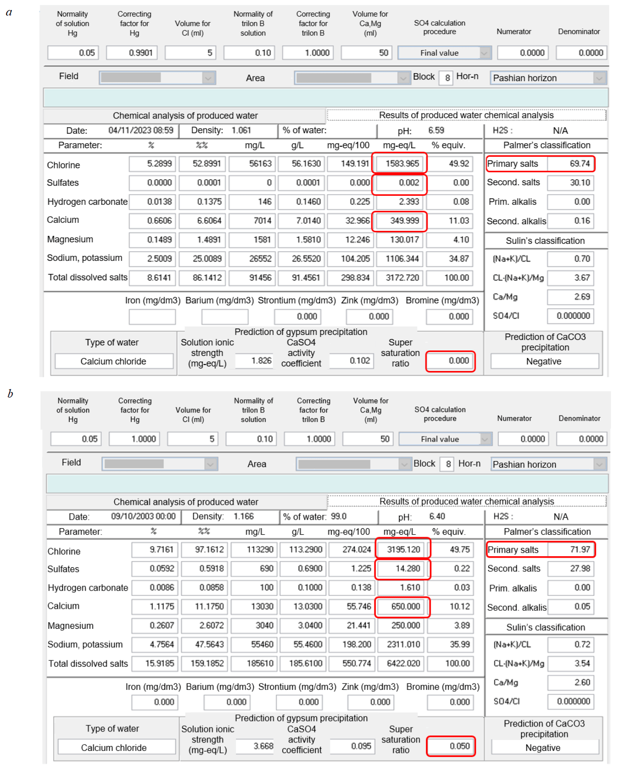
Fig.1. Results of water chemical analysis: for wells with leak-tight (a) and leaking (b) production casing
To assess distribution of the analyzed parameters by the field N areas, 14,318 well survey reports obtained from corporate databases for the 2000-2022 period were analyzed. The selected features included parameters characte-rizing water chemical composition, well perfor-mance, and well age.
Initially, distribution of each parameter was evaluated to analyze anomalies and outliers. Outliers are defined as data values that significantly deviate from the majority of other values in the dataset [44, 45]. The interquartile range (IQR) method [46] was selected for outlier detection.
Figure 2 shows a schematic representation of a range diagram, also known as a “box-and-whisker”. This type of diagram displays all quartiles of the source data. Quartile Q1 is the value that separates the first quarter of the dataset, meaning that 25 % of the data are less than this value, and 75 % are greater. Next is the median value (the second quartile, Q2) which divides the dataset into two halves, meaning that 50 % of the data are less than this value and 50 % are greater. The third quartile, Q3, is the value that separates three quarters of the dataset, meaning that 75 % of the data are less than this value, and 25 % are greater. The distance between the third and first quartiles is called the interquartile range. The plot also has “whiskers” that extend leftward from the first quartile and rightward from the third quartile. The length of each whisker is equal to one and a half of the interquartile range. Any data points located beyond the whiskers can be considered as outliers.
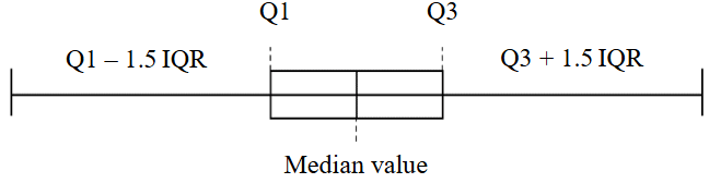
Fig.2. Range diagram
Based on the described approach, outliers were analyzed across the areas of the N field. To begin with, let's consider outliers for wells with a leak-tight production casing string. Features with the highest average proportion of outliers include water chemical analysis, namely the Ca/Mg ratio 0.19, sulfate content 0.15, and Cl–(Na+K)/Mg ratio 0.14.
As for parameters characterizing well performance, no outliers are observed, which indicates a reasonably good data representativeness. As for parameters characterizing water composition, the situation is not so straightforward. Features with proportion of outliers less than 10 % include water density, solution ionic strength, pH value, chloride content, bicarbonate content, calcium content, magnesium content, sodium content, total dissolved salts, (Na+K)/Cl ratio, and content of primary and secondary salts. Features with proportion of outliers over 10 % include CaSO4 activity coefficient, supersaturation ratio, sulfate content, Cl–(Na+K)/Mg ratio, Ca/Mg ratio, and content of secondary alkalis.
In the group of wells with a leaking casing string, the number of outliers is lower than in wells with a leak-tight casing string. Features with the highest proportion of outliers include content of secondary alkalis, fluid flow rate, and calcium concentration. In the entire dataset for wells with a casing leakage problem, the percentage of outliers does not exceed 10 %, which indicates sufficient dataset homogeneity.
The most interesting conclusions can be drawn for the dataset with a leak-tight casing string, which exhibits a higher percentage of outliers. It is possible that measurements were conducted incorrectly, and based on a number of parameters the well was classified as leaking, but all in all it was classified as leak-tight based on various studies and analyses. This discrepancy could be the reason for the outliers in the total dataset. The method proposed in this study allows for the analysis of multiple parameters and provides a correct assessment of well integrity.
The next step was filling the missing values. First, the missing values were filled using the previous value for each specific well, and then the remaining missing values for each specific well were filled from the bottom up, i.e., using the next subsequent value.
Following data preprocessing, a test for multicollinearity was performed using the Pearson correlation matrix. This matrix gives an insight into the strength and direction of the relationships between different features in the dataset [47].
The Pearson correlation matrix is based on the coefficients of linear correlation between all pairs of numerical variables in the dataframe:
where xi is the value of feature x in the i-th measurement; yi is the value of feature y in the i-th measurement; x‾ is the average value of feature x; y‾ is the average value of feature y; n is the number of measurements.
Figure 3 presents the Pearson correlation matrix as a heat map for the features selected to analyze their impact on the loss of production casing integrity: F1 – area code; F2 – well age at the time of the study; Y – casing condition; F3 – water density; F4 – ionic strength; F5 – CaSO4 activity coefficient; F6 – oversaturation ratio; F7 – pH; F8 – chloride; F9 – sulfates; F10 – bicarbonate; F11 – calcium; F12 – magnesium; F13 – sodium; F14 – total dissolved salts; F15 – (Na+K)/Cl ratio; F16 – Cl–(Na+K)/Mg ratio; F17 – Ca/Mg ratio; F18 – primary salts; F19 – secondary salts; F20 – secondary alkalis; F21 – liquid rate; F22 – oil flow rate; F23 – water cut; F24 – reservoir pressure; F25 – bottomhole pressure; F26 – number of workover operations. The linear correlation coefficients are displayed at the intersection of the horizontal and vertical axes.
The strongest direct correlation is observed between the features that characterize water chemical composition (Fig.3). Due to the impact of strong feature correlation on model training and its subsequent application, a decision was made to remove one feature from each pair of dependent features. The following features were removed from the training dataset: solution ionic strength, chloride content, calcium content, magnesium content, sodium content, and the Ca/Mg ratio.
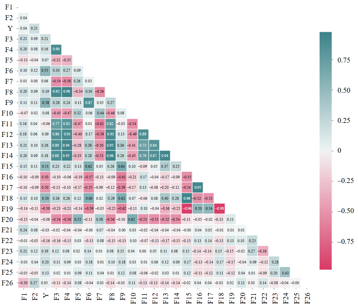
Fug.3. Feature correlation matrix in the dataset with regard to outlier processing
During the data processing stage, feature scaling was performed using the standardization method via the StandardScaler module from the scikit-learn library for the Python programming language [48]. Standardization is necessary due to the heterogeneity of feature values used for training. If standardization is not applied, the model will assume that features with larger values are more important than those with smaller values. The feature values were converted using the following equation:
where, zi – a standardized value; хi – initial value; μi – the average value (arithmetical average of all values); σi – standard feature deviation (measure of feature value spread relative to the average value).
At first, the average feature value is subtracted, which centers the distribution around zero. The second step is division by the standard deviation value, bringing the data to scale so that one standard deviation corresponds to a unit length. After standardization, we obtain a value that represents deviation of the original value from the average value in standard units.
A significant spread in values across different areas of the field is observed for a number of parameters, which is attributed to geological and physical characteristics of each production zone. In this context, the model training procedure was improved by incorporating the area feature and applying a knowledge transfer method [49]. This approach involves clustering of production zones based on water chemical analysis and using the silhouette method and the K-average algorithm. This made it possible to identify groups of similar production zones and consolidate data from zones with a small number of measurements with data from the analogous zones. The model was trained considering well clusters while recording the specific features of each production zone. This method increased prediction accuracy by 13 % and improved other model quality metrics. It also considered a specific production zone where the well was located when predicting production casing leakage.
To evaluate the importance of individual features and their ability to distinguish between leak-tight and leaking casings, the ROC-AUC (Receiver Operating Characteristic – Area Under the Curve) statistical analysis method was used [50]. It allows for evaluating feature importance based on their ability to distinguish between different classes. The process of AUC determining involves plotting of a ROC curve, which illustrates the relationship between True Positive Rate (TPR) and False Positive Rate (FPR) for a given feature. A higher AUC value indicates a better ability of the feature to distinguish between classes.
For each sample with a known feature value xi and a class mark yi (θ) {0, 1}, a binary classifier is defined based on the θ threshold value:
where yi(θ) is a predicted class for the i-th sample at a specified θ threshold; if хi ≥ θ, the sample is considered positive, if otherwise it is considered negative.
For each θ point, sensitivity (TPR) and specificity (FPR) are calculated:
where TP(θ) is a number of wells truly classified as leaking; FN(θ) is a number of well falsely classified as leak-tight; FP(θ) is a number of wells falsely classified as leaking; TN(θ) is a number of wells truly classified as leak-tight.
With variation of the classification threshold θ across the entire range of the feature values, a ROC curve is plotted – TPR(θ) versus FPR(θ). The integral under this curve defines the AUC metric:
where f is a proportion of false-positive classifications (FPR); TPR(f) is sensitivity at specified FPR.
In addition to determining feature importance, it is necessary to establish feature threshold values. One of the statistical parameters used for determining threshold values is Youden's index [51]:
The Youden’s index allows finding the threshold value at which the maximum difference between the TPR and the FPR is achieved in binary classification problem:
where θ* is an optimum classification threshold.
In addition to statistical methods, the ones based on machine learning models are also employed. One such method is SHAP analysis [52]. SHAP methods evaluate contribution of each feature to the model prediction, which helps identify the most significant factors affecting the result. This makes it a valuable tool for analyzing complex systems, such as well integrity diagnostics, where multiple factors contribute to the loss of integrity. Each point displayed on a SHAP plot represents the SHAP value for a specific case. The assembly of these points for each feature defines its distribution along the horizontal axis. Density of this distribution contains important information: broad dense areas on the plot indicate the range of SHAP values typical for the majority of measurements and reflect typical contribution of a feature. In contrast, narrow and elongated areas (the plot “tails”) correspond to rare but potentially strong impact, which can be associated with outliers or specific feature interactions. Low feature values are displayed in blue, and high values in red. Position of the points relative to the zero line shows the direction and strength of the feature impact. If the values are on the right side, a positive class is more likely to be predicted, meaning well integrity failure. If the points are on the left side, a negative class is likely to be predicted, meaning well tightness. Impact of each feature is assessed as the difference between the model prediction with this feature and without it, ensuring a fair distribution of contribution of each feature.
Model prediction with consideration of feature contribution according to SHAP-analysis is calculated as follows:
where ϕ0 is the base line; ϕi(x) is the SHAP value for the i-th feature; n is the number of features.
SHAP values are relative estimates of feature impact expressed in standardized units of deviation from the baseline ϕ0. However, for the practical application of the model, it is crucial to understand which absolute values correspond to the key transition points between leak-tight and leaking wells.
In particular, there is a threshold value for any feature at which the SHAP contribution is close to zero, meaning the model prediction does not tend either towards the positive or negative class. Such values can be interpreted as cutoff values that separate the areas of “low-risk” and “high-risk” of leakage.
To obtain threshold values, the standardized features were reconverted back to their original physical scale. Based on scaling of each feature, the value corresponding to a neutral SHAP contribution is calculated by the following equation:
where zi(0) is a standardized value at which the SHAP-contribution is equal to zero; zi(0)= 0; γi is an absolute threshold value.
The scientific novelty of this research consists in the development of an interpretable machine learning model based on the LightGBM algorithm [53] using SHAP analysis, which has been adapted for the first time to detecting production casing leakage. Unlike conventional implementations, LightGBM employs a tree growth strategy, which provides higher accuracy and training efficiency, and utilizes a histogram discretization method to accelerate computations and reduce memory consumption.
LightGBM is classified as a method of gradient boosting on decision trees. The model prediction is expressed as the sum of predictions from individual trees:
where T is a number of trees in the assembly; ft is a decision tree function built on the t-th iteration; F is the space of all possible decision trees; ki is the i’s feature vector.
SHAP analysis was applied as a post-processing method for the LightGBM model results to quantify the contribution of individual features to the model prediction. This enabled interpretation of the model performance and identification of key features that determine the probability of leakage.
The SHAP method calculates marginal contribution of each feature to the model prediction, considering all possible combinations of features. In this study, the feature importance was assessed based on the average absolute SHAP value across the entire dataset:
where ϕij is SHAP value of j feature for i measurement; N is a number of samples.
The higher the value of Ij, the stronger the impact of a feature on the model prediction, on average.
Results and discussion
Figure 4 shows an example of the ROC analysis for sulfate content. This feature effectively distinguishes between leaking and leak-tight wells, as the area value under ROC curve is 0.8 u.f. The red dot indicates the optimal threshold for this feature according to Youden’s index (2.08 mg-eq/l); wells with leaking casing are more often observed above this threshold, and wells with leak-tight casing are more often observed below it. The remaining features were analyzed in a similar manner. The results of the analysis are presented in Table 1.
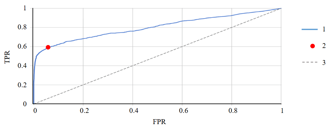
Fig.4. Example of sulfate content ROC analysis
1 – ROC-curve (AUC = 0.8); 2 – optimal threshold, AUC = 2.08; 3 – random guessing of actual model value
Table 1
AUC values and threshold values to distinguish between leak-tight and leaking wells based on ROC-AUC
|
Features |
AUC, f.u. |
Feature thresholds |
|
Sulfates, mg-eq/l |
0.802 |
2.082 |
|
Supersaturation ratio, f.u. |
0.776 |
0.114 |
|
(Na+K)/Cl, f.u. |
0.747 |
0.74 |
|
Primary salts, mg-eq/l |
0.741 |
73.68 |
|
Water cut, % |
0.647 |
93.83 |
|
Formation pressure, atm |
0.647 |
158 |
|
Water density, g/cm3 |
0.646 |
1.118 |
|
Well age, years |
0.645 |
36 |
|
Total dissolved salts, mg-eq/l |
0.627 |
5810.998 |
|
CaSO4 activity coefficient, f.u. |
0.619 |
0.101 |
|
Bottomhole pressure, atm |
0.58 |
114 |
|
Hydrocarbonate, mg-eq/l |
0.571 |
2.098 |
|
Number of workovers |
0.558 |
10 |
|
pH value, f.u. |
0.531 |
5.82 |
|
Fluid rate, m3/day |
0.503 |
13.145 |
|
Secondary alkalis, mg-eq/l |
0.467 |
0.04 |
|
Oil rate, m3/day |
0.368 |
0.004 |
|
Secondary salts, mg-eq/l |
0.257 |
38.62 |
|
Cl–(Na+K)/Mg, f.u. |
0.25 |
5.1 |
To interpret the predictive power of features, a qualitative scale was used [54], according to which AUC = 0.5 f.u. means classifier at the level of random guessing; AUC = 0.7-0.8 means acceptable; AUC = 0.8-0.9 means excellent; AUC > 0.9 means outstanding.
According to this scale, features such as sulfate content, solution supersaturation ratio, (Na+K)/Cl coefficient, and primary salts content are most important in statistical analysis, as the AUC value for the features is greater than 0.7. Features such as water content, formation pressure, and well age have a moderate impact on classification especially when combined with other factors. Features with the AUC value less than 0.6 f.u. have poor classification ability and are likely to play supporting role in well leakage prediction. However, this statistical analysis approach does not consider data nonlinear relationship and interaction between features, which may be critical for accurate prediction. ROC-AUC approach only evaluates the individual capacity of each feature to divide into classes, which limits its applicability in tasks such as well leakage detection.
Machine learning models combined with further SHAP analysis eliminate limitations of statistical methods.
Figure 5 shows SHAP analysis of feature importance calculated using equations (1) and (3). The features shown in the diagram are sorted by decreasing degree of impact on the model prediction.
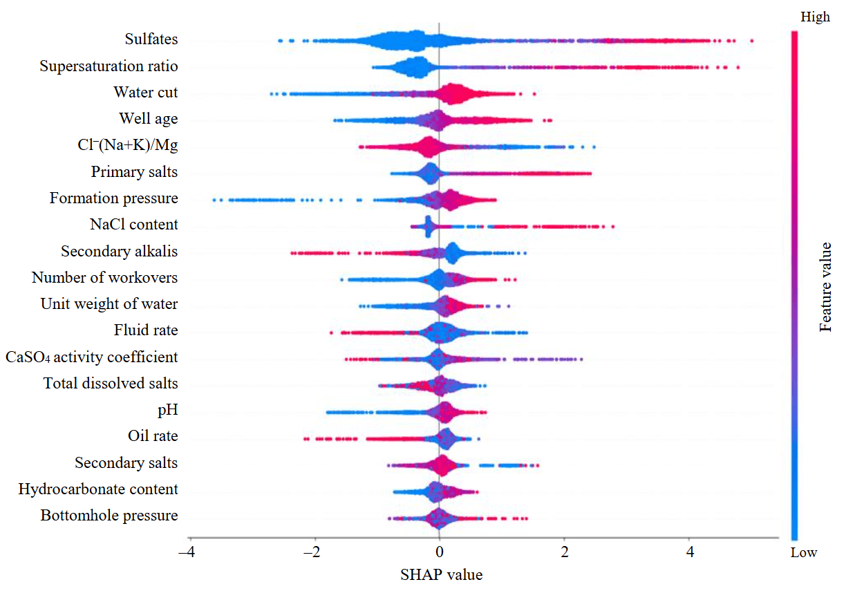
Fig.5. Evaluation of features impact on leakage occurrence
The following features have the greatest impact on the leak occurrence as per the LightGBM model, based on the average absolute SHAP value: SHAP value of sulfate content – 0.872; SHAP value of solution supersaturation ratio – 0.644; SHAP value of water cut – 0.436; SHAP value of well age at the time of study – 0.420; SHAP value of hydrochemical ratio for Cl–(Na+K)/Mg – 0.374.
In this study, absolute threshold values for features were determined from SHAP analysis using equation (2), changes in which can lead to an increased probability of leakage: sulfates – 2.36 mg-eq/l; supersaturation ratio – 0.10; water cut – 77.27 %; well age – 33 years; Cl–(Na+K)/Mg – 3.86 f.u.; primary salts – 69.50 mg-eq/l; formation pressure – 151.14 atm; (Na+K)/Cl – 0.70 f.u.; secondary salts – 30.29 mg-eq/l; number of workovers – 15; water density – 1.10 g/cm3; fluid rate – 27.04 m3/day; CaSO4 activity coefficient – 0.10 f.u.; total dissolved salts – 4776.53 mg-eq/l; pH value – 6.31 f.u.; oil rate – 3.13 m3/day; secondary alkalis – 0.11 mg-eq/l; hydrogen carbonate – 2.19 mg-eq/l; bottomhole pressure – 95.86 atm.
Sulfates and the supersaturation ratio have the greatest impact on predicting leakage, with only a slight difference in the values of the features (Table 1). In both cases, primary salts, well age, water cut, and formation pressure are also highly important. According to ROC-AUC statistical analysis, the hydrochemical ratio Cl–(Na+K)/Mg has the lowest impact on occurrence of leakage, while as per SHAP analysis, this feature is fifth in the order of importance. That is because SHAP analysis provides more accurate and interpretable threshold values, as it considers nonlinearities and combinations of features that are not detectable in simple ROC-AUC statistical analysis.
Figure 6 shows interpretation diagrams for five features that have the greatest impact on predicting well leakage.
The sulfate content value at which the SHAP value is neutral is 2.36 mg-eq/l (Fig.6, a), i.e., the values below this level reduce the likelihood of leakage, while the values above this level increase it.
As for supersaturation ratio, the threshold value is 0.1 (Fig.6, b). Higher values are more often observed in wells with leaking casing. As part of this study, the value of the supersaturation ratio in the terrigenous Devonian water was calculated. On average, it is 0.017, while the supersaturation ratio for the Lower and Middle Carboniferous ranges between 0 and 2.48, with an average of 0.69. Consequently, it can be concluded that as the supersaturation ratio in the water sample obtained from the well increases, there is high probability of fluid influx from the overlying horizons, from the Carboniferous sediments, in particular.
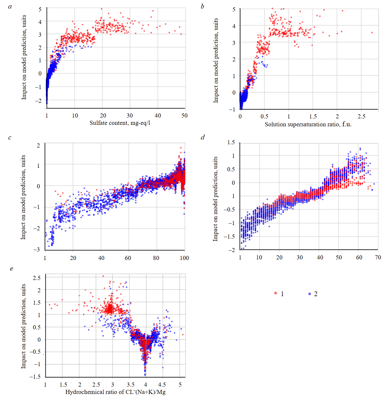
Fig.6. Diagrams of features impact on the casing leakage occurrence: а – sulfate content; b – supersaturation ratio; c – water cut; d – well age; e – hydrochemical ratio of Cl–(Na+K)/Mg
1 – leaking well; 2 –leak-tight well
As the water cut value increases, the probability of predicting well leakage also increases (Fig.6, c). The water cut value at which the SHAP value reaches its threshold is 77.27 %.
As the well age increases, the probability of predicting well leakage also increases (Fig.6, d). The well age threshold value according to SHAP analysis is 33 years.
As the value of hydrochemical ratio of Cl–(Na+K)/Mg decreases, the probability of casing leakage increases (Fig.6, e). If the value of the hydrochemical ratio of Cl–(Na+K)/Mg is around 3.86, there is a boundary zone between cases with leak-tight and leaking casings. As part of this study, the value of hydrochemical ratio of Cl–(Na+K)/Mg in the terrigenous Devonian water was calculated – on average it is 4.08, while the value of Cl–(Na+K)/Mg in the Lower and Middle Carboniferous water varies between 0.89 and 3.17, with an average of 2.40. When the value of the hydrochemical ratio of Cl–(Na+K)/Mg in a sample obtained from the well decreases, there is a high probability of fluid influx from the overlying horizons, from the Carboniferous sediments, in particular.
Comparison of the threshold values determined by statistical methods and machine learning models with further SHAP analysis is presented in Table 2.
Table 2
Comparison of features threshold values as per ROC-AUC method and SHAP analysis
|
Features |
Threshold value |
Difference between values, % |
|
|
ROC-AUC |
SHAP |
||
|
Sulfates, mg-eq/l |
2.082 |
2.36 |
–13 |
|
Supersaturation ratio, f.u. |
0.114 |
0.1 |
12 |
|
(Na+K)/Cl, f.u. |
0.74 |
0.7 |
5 |
|
Primary salts, mg-e/l |
73.68 |
69.5 |
6 |
|
Water cut, % |
93.83 |
77.27 |
18 |
|
Formation pressure, atm |
158 |
151.14 |
4 |
|
Water density, g/cm3 |
1.118 |
1.1 |
2 |
|
Well age, years |
36 |
33 |
8 |
|
Total dissolved salts, mg-eq/l |
5810.998 |
4776.53 |
18 |
|
CaSO4 activity coefficient, f.u. |
0.101 |
0.1 |
1 |
|
Bottomhole pressure, atm |
114 |
95.86 |
16 |
|
Hydrocarbonate, mg-eq/l |
2.098 |
2.19 |
–4 |
|
Number of workovers |
10 |
15 |
–50 |
|
pH value, f.u. |
5.82 |
6.31 |
–8 |
|
Fluid rate, m3/day |
13.145 |
27.04 |
–106 |
|
Secondary alkalis, mg-eq/l |
0.04 |
0.11 |
–175 |
|
Oil rate, m3/day |
0.004 |
3.13 |
–78,150 |
|
Secondary salts, mg-eq/l |
38.62 |
30.29 |
22 |
|
Cl–(Na+K)/Mg, f.u. |
5.1 |
3.86 |
24 |
For 12 features, ROC-AUC statistical analysis shows higher threshold values compared to SHAP analysis (Table 2), e.g., for the supersaturation ratio those are 0.114 and 0.1, respectively. Conversely, for seven features ROC-AUC demonstrates lower values, e.g., for sulfate content – 2.082 and 2.36 respectively. In the first case, we can say that SHAP analysis focuses on recognizing even small changes in features. In the second case, ROC-AUC analysis attempts to cover the entire range of values that may be important for classification. For oil recovery rate there are significant differences in the threshold values depending on the analysis method. This is probably due to the fact that this feature has a nonlinear impact on the leakage prediction, and the ROC-AUC approach was unable to detect the relationship between the values of this feature and the leakage occurrence in the well.
Unlike previously used machine learning models and statistical methods, the proposed approach provides not only high prediction accuracy, but also interpretation of the threshold values of key features, such as sulfate content, supersaturation ratio, water cut, and well age. It also demonstrates high importance of previously underestimated features identified by SHAP analysis, which was impossible using conventional ROC-AUC analysis.
Conclusion
In this study, applicability of machine learning methods for detecting well casing integrity issues was analyzed.
SHAP analysis allows identification of absolute threshold values of key features. For example, sulfate content threshold exceeding of which will likely result in casing leakage, is 2.36 mg-eq/l, supersaturation ratio threshold is 0.1, and water cut threshold is 77.27 %.
ROC-AUC analysis shows that some features, such as sulfate content and supersaturation ratio, exhibit high ability to distinguish between leak-tight and leaking wells. However, SHAP analysis provides a more in-depth model interpretation by taking into consideration nonlinearity and synergistic effects between features. This makes the SHAP analysis a valuable tool for analyzing complex systems, such as well operation, where multiple factors affect leakage occurrence. Thus, combination of machine learning methods and SHAP analysis increases prediction accuracy and reliability of results, providing a better basis for decision-making.
The practical significance of this study lies in the applicability of interpretable machine learning models to various tasks in the oil and gas industry, including monitoring of production casing integrity. This approach will facilitate prompt identification of risk zones and will mitigate environmental risks and economic losses during well logging and production operations.
References
- Chernenko A.V., Lyshko G.N. Prevention of Formation Fluids Flows in Anullar Space Based on Mathematical Modeling of Processes in the Well. Neft. Gas. Novacii. 2018. N 3 (208), p. 30-33 (in Russian).
- Nabiullin A.Sh., Sinitsyna T.I., Vorontsov S.Yu. Studying the causes of casing leakages in production wells. Developing preventive methods for casing protection. Exposition Oil Gas. 2023. Iss. 8, p. 88-93 (in Russian). DOI: 10.24412/2076-6785-2023-8-88-93
- Anikeev D.P., Zakirov S.N., Anikeeva E.S., Lysenko A.D. Well leakage is a global problem, not a local one. Actual Problems of Oil and Gas. 2019. Iss. 4 (27), p. 14 (in Russian). DOI: 10.29222/ipng.2078-5712.2019-27.art15
- Trunov E.I., Ozdoeva A.Kh., Blotskaya A.I. et al. New approaches to the application of the acoustic method for continuous monitoring of well cementing integrity. Oil Industry Journal. 2024. N 2, p. 38-42 (in Russian). DOI: 10.24887/0028-2448-2024-2-38-42
- Sharipov A.F., Volkov A.N. System for control and appraisal of well gas-condensate tests quality. Vesti gazovoy nauki. 2016. N 4 (28), p. 173-180 (in Russian).
- Valiullin R.A., Sharafutdinov R.F., Fedotov V.Y. et al. The thermal convection study of behind-casing flow directed from up to down on a well model with induction heater. Bulletin of Bashkir University. 2017. Vol. 22. N 2, p. 325-329 (in Russian).
- Patidar A.K., Joshi D., Dristant U., Choudhury Y. et al. A review of tracer testing techniques in porous media specially attributed to the oil and gas industry. Journal of Petroleum Exploration and Production Technology. 2022. Vol. 12. Iss. 12, p. 3339-3356. DOI: 10.1007/s13202-022-01526-w
- Batista G. dos S., Takimi A.S., da Costa E.M. Chemical Changes in the Composition of Oil Well Cement with Core/Shell Nanoparticle Addition under CO2 Geological Storage Conditions. Energy & Fuels. 2024. Vol. 38. Iss. 23, p. 22947-22958. DOI: 10.1021/acs.energyfuels.4c03686
- Azamatov M.A., Shorokhov A.N. Production casing leakage determining method. Nedropolzovanie XXI vek. 2015. N 6 (56), p. 43-47 (in Russian).
- Shcherbakova K.O. The problem of high water cut in the products of horizontal wells. Proceedings of higher educational establishments. Geology and Exploration. 2022. Vol. 64. N 6, p. 29-38 (in Russian). DOI: 10.32454/0016-7762-2022-64-6-29-38
- Jabarov K.A. Mathematical modeling the processes of behind-casing fluid movement in the wells during waiting on cement. Oil Industry Journal. 2019. N 5, p. 67-71 (in Russian). DOI: 10.24887/0028-2448-2019-5-67-71
- Burkova A.A. Application of a new technology for repair and insulation works. Construction of oil and gas wells on land and sea. 2022. N 8 (356), p. 39-44 (in Russian). DOI: 10.33285/0130-3872-2022-8(356)-39-44
- Freiman O.A., Eremin N.A. Development of a methodology for predicting reservoir properties of oil using machine learning methods. Exposition Oil Gas. 2023. Iss. 7, p. 118-120 (in Russian). DOI: 10.24412/2076-6785-2023-7-118-120
- Tadjer A., Hong A., Bratvold R.B. Machine learning based decline curve analysis for short-term oil production forecast. Energy Exploration & Exploitation. 2021. Vol. 39. Iss. 5, p. 1747-1769. DOI: 10.1177/01445987211011784
- Pashali A.A., Azbukhanov A.F., Sukharev K.V., Topolnikov A.S. The pressure levels restoration at the pump suction on oil producing wells by the use of machine learning methods. Petroleum Engineering. 2022. Vol. 20. N 6, p. 165-172 (in Russian). DOI: 10.17122/ngdelo-2022-6-165-172
- Liang Xue, Yuetian Liu, Yifei Xiong et al. A data-driven shale gas production forecasting method based on the multi-objective random forest regression. Journal of Petroleum Science and Engineering. 2021. Vol. 196. N 107801. DOI: 10.1016/j.petrol.2020.107801
- Evseenkov A.S., Guz V.S., Shpetny D.N., Yudin E.V. Short-term forecasting of well flow rate based on probabilistic approach. Oil Industry Journal. 2023. N 2, p. 78-82 (in Russian). DOI: 10.24887/0028-2448-2023-2-78-82
- Arief I.H., Tao Yang. A Machine-Learning Approach to Predict Gas-Oil Ratio Based on Advanced Mud Gas Data. Petrophysics. 2024. Vol. 65. Iss. 4, p. 433-454.
- Negash B.M., Yaw A.D. Artificial neural network based production forecasting for a hydrocarbon reservoir under water injection. Petroleum Exploration and Development. 2020. Vol. 47. Iss. 2, p. 383-392. DOI: 10.1016/S1876-3804(20)60055-6
- Gabitova S.I., Davletbakova L.A., Klimov V.Yu. et al. A new method of decline curve forecasting for project wells on the base of machine learning algorithms. PROneft. Professionals about Oil. 2020. N 4 (18), p. 69-74 (in Russian). DOI: 10.7868/S2587739920040102
- Werneck R. de O., Prates R., Moura R. et al. Data-driven deep-learning forecasting for oil production and pressure. Journal of Petroleum Science and Engineering. 2022. Vol. 210. N 109937. DOI: 10.1016/j.petrol.2021.109937
- Xuanyi Song, Yuetian Liu, Liang Xue et al. Time-series well performance prediction based on Long Short-Term Memory (LSTM) neural network model. Journal of Petroleum Science and Engineering. 2020. Vol. 186. N 106682. DOI: 10.1016/j.petrol.2019.106682
- Ahmadi M.A., Soleimani R., Lee M. et al. Determination of oil well production performance using artificial neural network (ANN) linked to the particle swarm optimization (PSO) tool. Petroleum. 2015. Vol. 1. Iss. 2, p. 118-132. DOI: 10.1016/j.petlm.2015.06.004
- Pechko K.A., Senkin I.S., Belonogov E.V. Well modeling using machine learning methods for integrated modeling. PROneft. Professionals about Oil. 2022. Vol. 7. N 2 (23), p. 114-120 (in Russian). DOI: 10.51890/2587-7399-2022-7-2-114-120
- Vikara D., Khanna V. Application of a Deep Learning Network for Joint Prediction of Associated Fluid Production in Unconventional Hydrocarbon Development. Processes. 2022. Vol 10. Iss. 4. N 740. DOI: 10.3390/pr10040740
- Ng C.S.W., Ghahfarokhi A.J., Amar M.N. Application of nature-inspired algorithms and artificial neural network in waterflooding well control optimization. Journal of Petroleum Exploration and Production Technology. 2021. Vol. 11. Iss. 7, p. 3103-3127. DOI: 10.1007/s13202-021-01199-x
- Martyushev D.A., Ponomareva I.N., Zakharov L.A., Shadrov T.A. Application of machine learning for forecasting formation pressure in oil field development. Bulletin of the Tomsk Polytechnic University. Geo Аssets Engineering. 2021. Vol. 332. N 10, p. 140-149 (in Russian). DOI: 10.18799/24131830/2021/10/3401
- Ponomarev R.Yu., Migmanov R.R., Ziazev R.R. Assessment of the possibilities of using hybrid modeling to optimize the production potential of an oil and gas field. Exposition Oil Gas. 2023. Iss. 5, p. 64-68 (in Russian). DOI: 10.24412/2076-6785-2023-5-64-68
- Mekhonoshin R.O., Vildanov T.F., Kordik K.E. et al. Prediction of incidents occurrence at injection wells using machine learning algorithms. Oilfield engineering. 2023. N 9 (657), p. 16-21 (in Russian). DOI: 10.33285/0207-2351-2023-9(657)-16-21
- Chernikov A.D., Eremin N.A., Stolyarov V.E. et al. Application of artificial intelligence methods for identifying and predicting complications in the construction of oil and gas wells: problems and solutions. Georesources. 2020. Vol. 22. N 3, p. 87-96. DOI: 10.18599/grs.2020.3.87-96
- Shibaev A.A., Shrago I.L., Vasinkin I.A., Chernyshov A.S. Application of machine learning methods in the task of analysis of anomal behavior of technological features, in the classification of technological operations, of the well construction cycle. Burenie i neft. 2023. N 7-8, p. 28-31 (in Russian).
- Dexin Ma, Hongbo Yang, Zhi Yang et al. An Intelligent Method for Real-Time Surface Monitoring of Rock Drillability at the Well Bottom Based on Logging and Drilling Data Fusion. Processes. 2025. Vol. 13. Iss. 3. N 668. DOI: 10.3390/pr13030668
- Shalyapin D.V., Bakirov D.L., Fattakhov M.M. et al. The applying of machine learning methods to improve the quality of well casing. Oil and Gas Studies. 2020. N 5 (143), p. 81-93 (in Russian). DOI: 10.31660/0445-0108-2020-5-81-93
- Shlykov S.V. Application of machine learning methods to automate processes in the oil and gas industry. Transport and storage of Oil Products and Hydrocarbons. 2023. N 2, p. 46-53 (in Russian). DOI: 10.24412/0131-4270-2023-2-46-53
- Maiorov K.N. Application of machine learning algorithms for solving problems in the oil and gas sector. Intelligent Systems in Manufacturing. 2021. Vol. 19. N 3, p. 55-64 (in Russian). DOI: 10.22213/2410-9304-2021-3-55-64
- Sakhnyuk V.I., Novickov E.V., Sharifullin A.M. et al. Machine learning applications for well-logging interpretation of the Vikulov Formation. Georesources. 2022. Vol. 24. N 2, p. 230-238 (in Russian). DOI: 10.18599/grs.2022.2.21
- Rammay M.H., Abdulraheem A. PVT correlations for Pakistani crude oils using artificial neural network. Journal of Petroleum Exploration and Production Technology. 2017. Vol. 7. Iss. 1, p. 217-233. DOI: 10.1007/s13202-016-0232-z
- Salem A.М., Yakoot M.S., Mahmoud O. A novel machine learning model for autonomous analysis and diagnosis of well integrity failures in artificial-lift production systems. Advances in Geo-Energy Research. 2022. Vol. 6. N 2, p. 123-142. DOI: 10.46690/ager.2022.02.05
- Sadiki N., Jang D.-W. Estimation of Hydraulic and Water Quality Features Using Long Short-Term Memory in Water Distribution Systems. Water. 2024. Vol. 16. Iss. 21. N 3028. DOI: 10.3390/w16213028
- Xiaohui Yan, Tianqi Zhang, Wenying Du et al. A Comprehensive Review of Machine Learning for Water Quality Prediction over the Past Five Years. Journal of Marine Science and Engineering. 2024. Vol. 12. Iss. 1. N 159. DOI: 10.3390/jmse12010159
- Ishkulov I.M., Vafin R.R., Takhauov D.D. et al. Production casing leak detection methods revisited. Oil Industry Journal. 2024. N 7, p. 56-60 (in Russian). DOI: 10.24887/0028-2448-2024-7-56-60
- Ishkulov I.M., Tahauov D.D., Vafin R.R. et al. Well string leak detection using machine learning models. Petroleum Engineering. 2024. Vol. 22. N 4, p. 260-267 (in Russian). DOI: 10.17122/ngdelo-2024-4-260-267
- Xianlin Ma, Mengyao Hou, Jie Zhan, Zhenzhi Liu. Interpretable Predictive Modeling of Tight Gas Well Productivity with SHAP and LIME Techniques. Energies. 2023. Vol. 16. Iss. 9. N 3653. DOI: 10.3390/en16093653
- Smiti A. A critical overview of outlier detection methods. Computer Science Review. 2020. Vol. 38. N 100306. DOI: 10.1016/j.cosrev.2020.100306
- Kiani R., Wei Jin, Sheng V.S. Survey on extreme learning machines for outlier detection. Machine Learning. 2024. Vol. 113. Iss. 8, p. 5495-5531. DOI: 10.1007/s10994-023-06375-0
- Dash C.S.K., Behera A.K., Dehuri S., Ghosh A. An outliers detection and elimination framework in classification task of data mining. Decision Analytics Journal. 2023. Vol. 6. N 100164. DOI: 10.1016/j.dajour.2023.100164
- Morais É.T., Barberes G.A., Souza I.V.A.F. et al. Pearson Correlation Coefficient Applied to Petroleum System Characterization: The Case Study of Potiguar and Reconcavo Basins, Brazil. Geosciences. 2023. Vol. 13. Iss. 9. N 282. DOI: 10.3390/geosciences13090282
- Thippa Reddy G., Swarna Priya R.M., Parimala M. et al. A deep neural networks based model for uninterrupted marine environment monitoring. Computer Communications. 2020. Vol. 157, p. 64-75. DOI: 10.1016/j.comcom.2020.04.004
- Ishkulov I.M., Safarov А.Kh., Fattakhov I.G., Dyakonov А.А. Application of knowledge transfer method for predicting wells integrity failure. Oilfield engineering. 2025. № 5 (677), p. 24-28 (in Russian).
- Chicco D., Jurman G. The Matthews correlation coefficient (MCC) should replace the ROC AUC as the standard metric for assessing binary classification. BioData Mining. 2023. Vol. 16. N 4. DOI: 10.1186/s13040-023-00322-4
- Starovoitov V.V., Golub Y.I. Comparative study of quality estimation of binary classification. Informatics. 2020. Vol. 17. N 1, p. 87-101 (in Russian). DOI: 10.37661/1816-0301-2020-17-1-87-101
- Ishkulov I., Vafin R., Takhauov D. еt al. Innovative approach to diagnostics of well integrity using machine learning. Norwegian Journal of Development of the International Science. 2024. N 144, p. 29-34. DOI: 10.5281/zenodo.14169109
- Guolin Ke, Qi Meng, Finley T. et al. LightGBM: A Highly Efficient Gradient Boosting Decision Tree. Advances in Neural Information Processing Systems 30: 31st Annual Conference on Neural Information Processing Systems (NIPS 2017), 4-9 December 2017, Long Beach, CA, USA. Curran Associates Inc., 2018, p. 3147-3155. DOI: 10.5555/3294996.3295074
- Hosmer D.W., Lemeshow S. Applied Logistic Regression. Wiley, 2000, p. 392. DOI: 10.1002/0471722146