


Geomagnetic data and the new national models for inclinometry of horizontal oil and gas wells in the Far North and Arctic shelf regions
- 1 — Ph.D., Dr.Sci. Director Trofimuk Institute of Petroleum Geology and Geophysics, SB RAS ▪ Orcid
- 2 — Ph.D. Head of Laboratory Trofimuk Institute of Petroleum Geology and Geophysics, SB RAS ▪ Orcid
- 3 — Ph.D., Dr.Sci. Professor Kazan (Volga Region) Federal University ▪ Orcid
- 4 — Expert Russian Energy Agency, Ministry of Energy of Russia ▪ Orcid
- 5 — Ph.D. Head of Sector Geophysical Center of the RAS ▪ Orcid
- 6 — Ph.D., Dr.Sci. Director Geophysical Center of the RAS ▪ Orcid
Abstract
This article addresses the important challenge of ensuring accurate inclinometer measurements during the construction of directional and horizontal wells in the Far North and Arctic shelf of Russia. In these regions, traditional inclinometer methods based on accelerometers and magnetometers face significant challenges due to significant changes in the geomagnetic field (magnetic storms, secular variations, and other disturbances). Wellbore azimuth measurement errors due to geomagnetic field distortions lead to risks of deviation from the planned trajectory, resulting in financial and techno-logical losses. A detailed analysis has been conducted and requirements for the use of up-to-date geomagnetic data and high-precision mathematical models have been formulated, providing the basis for correcting inclinometer measurements during horizontal drilling at critical latitudes. It is not enough to use outdated or global models (IGRF) in order to compensate for external magnetic disturbances in the Arctic: local, regularly updated high-resolution models (similar to HRGM, IFR-1, IFR-2), taking into account the regional particularities and local lithospheric magnetic anomalies, are needed. The national geomagnetic models (CAMPUS-C, CAMPUS-A, CAMPUS-CA, DIF-1), developed by the Geophysical Center of the RAS and the Institute of Petroleum Geology and Geophysics SB RAS for the oil and gas industry, are presented, and for the first time their applicability as a replacement for foreign models (BGGM/HDGM) for directional drilling tasks in the Arctic conditions is substantiated. The new national geomagnetic models and a detailed justification for the optimal number and location of geomagnetic observatories necessary to ensure reliable monitoring of the magnetic environment are proposed. The application of such specialized models and data helps mitigate the effects of geomagnetic interference, ensuring reliable determination of the drilling tool’s spatial position during horizontal drilling. This helps optimize drilling processes and improve the safety and efficiency of Arctic field development, which is of strategic importance for the Russian Federation.
This work was conducted in the framework of budgetary funding of the Institute of Petroleum Geology and Geophysics SB RAS (N FWZZ-2026-0051) and the Geophysical Center of the RAS (N 75-00444-26-01).
Introduction
Oil production in Russia by the end of 2024 will amount to 520-530 million tons, equivalent to 10.3-10.5 million barrels per day. Gas production in Russia reached 685 billion m3 [1]. Maintaining the current level of hydrocarbon production is one of the priorities outlined in the Energy Strategy of the Russian Federation up to 2050 [2]. It is planned that maintaining this level will be ensured by developing fields in the Far North and the Arctic, where oil production is projected to increase by up to 25%. By 2035, production is expected to reach at least 200 million tons of oil and 1 trillion m3 of gas [3].
About 60% of proven hydrocarbon reserves are concentrated in new Arctic projects located north of 60°N [4]. Due to complex logistics, underdeveloped transportation infrastructure, and harsh natural conditions, the development of these fields is economically feasible using modern drilling technologies for high-flow horizontal and directional wells ranging from 4-5 to over 10 km in length. However, in the Far North, drilling is characterized by a dense well network due to limited space for drilling equipment. This requires high-precision wellbore positioning [5], which is achieved with the help of underground navigation and well trajectory control techniques. For example, when extracting oil and gas on the shelf of the Sea of Okhotsk, where record-long subhorizontal wells are being drilled, hitting a given point underground is ensured at a distance of up to 15 km from the wellhead [5, 6].
Specific difficulties of inclinometry during horizontal drilling in the Far North
The influence of geomagnetic factors on inclinometry at high latitudes
Russian Arctic fields are located at latitudes above 60°, which creates additional difficulties when drilling wells using magnetometric inclinometers. The main difficulties are related to [7]: the obvious decrease of the geomagnetic field horizontal component magnitude towards the poles; magnetic storms and substorms caused by solar flares and coronal mass ejections; the north magnetic pole drift at a speed of 55-60 km/year; high-latitude auroral disturbances within the auroral zone (60-75° latitude).
Critical increase in sensitivity to geomagnetic interference in horizontal drilling
In horizontal drilling, the accuracy of inclinometer measurements is even more critical than in directional drilling, as the results of measurements carried out by borehole inclinometers become extremely sensitive to magnetic interference [8]. As the borehole spatial trajectory approaches a true horizontal direction, the gravity field vertical component (measured by accelerometers) becomes minimal and practically uninformative, while the dependence on the correct determination of the azimuth increases exponentially.
When drilling horizontally in the west-east direction (as the magnetic azimuth is close to 90° and 270°), the horizontal magnetic field component in this direction is significantly weaker, making the tool extremely sensitive to interference. Even small variations in the magnetic field lead to azimuth errors of up to several degrees, which can cause the well to deviate from the planned trajectory by tens of meters at depth.
The accuracy of azimuth measurements by inclinometers in these latitudes decreases, and the error can increase to ±3-8° (compared to ±0.5-1.5° in temperate latitudes) [9]. This is two to three times higher than the permissible values when drilling high-flow horizontal wells in dense network conditions.
The magnetic pole drift and its consequences
At northern latitudes the increase in error of the inclinometric azimuth measurements is due to the alternation in the characteristics of the Earth’s magnetic field subject to external effects caused by space weather phenomena. During magnetic storms and substorms geomagnetic navigation becomes difficult. The higher the latitude, the more intense these effects are, as the dipole configuration of the magnetosphere directs the magnetic field lines toward the poles, and the disturbance fields in the polar regions are significantly more intense than at low latitudes [9].
The intensity of the magnetic field drift in the Arctic is determined by a displacement of the magnetic pole by 55-60 km per year and a change in magnetic declination up to 0.2-0.3° per year (in total the deviation from the declination can reach 1.5° for 5 years [10]). In this case, the measurement error of the azimuth angle increases to 3-8° with standard measurements, and the additional error due to the Earth’s magnetic field drift is ±0.5-1.2° [9]. As a result, the total wellbore positioning error at 3000 m depth reaches 15-30 m in lateral deviation, and at a distance of 8000 m from the wellhead – 40-80 m [11]. This is critical for horizontal wells for which the permissible wellbore deviations are ±10m vertically and ±20m horizontally, and in complicated conditions (for example, near salt domes or when developing low-permeability reservoirs) up to ±5m.
Exceeding the design limits of a wellbore during horizontal drilling is associated with the risk of accidents when crossing adjacent wells and the wellbore exiting the productive formation. This leads to economic losses of 10-15% (well re-drilling), which amounts to \$0.5-2 million (average losses per well). At fields in the Far North and the Arctic shelf, where wells are 8-15 km long, drilling costs reach \$30-50 million. Errors in drilling high-flow wells in these areas can lead to the complete loss of investment in field development. Therefore, to minimize risks, it is important to account for variations in the Earth’s magnetic field, continuously monitor the magnetic field at the drilling site with high precision to ensure current reference values, and continuously adjust the magnetometer measurements installed in the drill string [12].
It’s important to note that there are downhole instruments that are not susceptible to magnetic interference. These instruments include gyroscopic systems (Gyro-While-Drilling, GWD) used in the wellbore trajectory adjustment. However, magnetometric systems are more cost-effective than gyroscopic ones, provided that proper azimuth measurement correction is applied. Therefore, borehole inclinometers based on the architecture of using three accelerometers and three magnetometers have become widely used in oil and gas fields not only in Russia but also abroad [12, 13]. Table 1 shows a comparison of the accuracy characteristics of inclinometry technologies at high latitudes.
Table 1
Accuracy characteristics of inclinometry technologies at high latitudes
|
Parameter |
Magnetic systems (without correction) |
Gyroscopic systems |
Magnetic systems+ HRGM/IFR |
|
Accuracy at 70° N |
0.1-0.3° (±2-5° during storms) |
0.1-0.5° |
0.05-0.15° |
|
Cost (per well) |
\$50,000-100,000 |
\$500,000-800,000 |
\$100,000-200,000 |
|
Continuity |
Correction required |
Limited (4-6 h) |
Full |
|
Demand for stops |
No |
Yes |
No |
The architecture of inclinometer sensors, common at Russian fields, includes three accelerometers and three magnetometers, providing recording of three components of the Earth’s gravitational and magnetic field vectors [14]. This architecture enables highly accurate inclinometer data acquisition under normal measurement conditions. In boreholes, inclinometers are susceptible to magnetic interference caused by magnetization of the drill string and bottomhole assembly (BHA) components, as well as magnetization of adjacent well casings made of magnetic materials. To ensure accuracy in underground navigation when drilling high-flow directional and horizontal wells, in addition to using non-magnetic metals and alloys in the BHA, mathematical methods for inclinometer data correction are also used.
Without the use of mathematical correction algorithms, inclinometers are not capable of providing the rated accuracy in downhole conditions (as part of a BHA), and the error in determining the azimuth can exceed ±20°, whereas the accuracy characteristics of downhole instruments are key to ensuring oil and gas recovery rates [14]. Therefore, when working with magnetometric inclino-meters, it is necessary to use specialized algorithms for mathematical data processing that use three-component measurements of the Earth’s magnetic field as input information, as well as the true values of the geomagnetic field parameters at the measurement point.
The system for correcting the borehole trajectory of a drilling oil and gas well using geomagnetic data is based on comparing the results of measurements from a magnetometer placed in the non-magnetic part of the BHA with reference values obtained from a geomagnetic field model or from direct field measurements in the drilling area [15, 16]. During horizontal drilling, the correction algorithms become extremely sensitive to the errors in magnetic field values, requiring the use of high-frequency data (1-minute-sampled or even continuous measurements) instead of traditional updates on a daily basis [16].
There are several methods for determining the parameters of the Earth’s geomagnetic field: using a mathematical model for location coordinates, direct measurements at the measurement point, and data from magnetic observatories. In practice, the primary source of geomagnetic data is the mathematical models of the Earth’s magnetic field.
According to the classification given by the Industry Steering Committee on Wellbore Survey Accuracy (ISCWSA), the current mathematical models of the Earth’s geomagnetic field are divided into five resolution categories based on the quality of their description of the internal field (Table 2).
Table 2
Classification of the Earth’s magnetic field models (ISCWSA)
|
Category |
Description |
Examples |
|
LRGM (Low Resolution) |
Main field; range of 40,000-4000 km; updated once every 5 years |
IGRF-14, WMM-2025, CGRF |
|
SRGM (Standard Resolution) |
Main and large-scale lithospheric field; updated annually |
BGGM, MVSD, CHAOS-8, WMMHR-2025 |
|
HRGM (High Resolution) |
Main field + regional magnetic anomalies; range up to ~28km; updated annually |
HDGM, MVHD, BGGM-HD, IZMIRAN, CAMPUS-CA |
|
IFR-1 (In-Field Referencing) |
Main field + regional and local anomalies; range up to first kilometers; observatory data at a distance up to 200km |
IFR-1 (BGS), DIF-1 (IPGG SB RAS) |
|
IFR-2 / IIFR (Interpolated IFR) |
IFR-1 with the integration of 1-minute-sampled data from the observatory; updated in real time |
HDGM-RT IFR-2, BGS IFR-2 |
For a long time, for drilling horizontal, subhorizontal and directional wells, data from IGRF (International Geomagnetic Reference Field) and BGGM/HDGM (BGS Global Geomagnetic Model/High Definition Geomagnetic Model) models have been used in Russian oil fields. IGRF has low spatial resolution and an update frequency of approximately once every 5 years, whereas BGGM/HDGM has high resolution and is updated annually. However, Russia lacked its own fully functional geomagnetic databases for the fuel and energy sector, capable of covering all northern fields. Since January 1, 2023, foreign models have not been officially supplied to Russia, and internet access has been blocked. Therefore, developing its own models of the Earth’s geomagnetic field has become critically important for the Russian fuel and energy sector [17].
The need for such a procedure is due to the fact that inclinometric measurements are performed under the influence of parasitic magnetic fields, which significantly distort the determination of azimuth and magnetic deflector. The main sources of geomagnetic fields and associated errors are listed in Table 3.
Table 3
The main sources of errors of a magnetic inclinometer
|
Error type |
Cause |
|
Misalignment |
|
|
Sensors related to the body |
Manufacturing tolerances or incomplete calibration |
|
Instruments relative to the borehole axis as part of a non-magnetic BHA |
Poor or no alignment |
|
Column relative to the wellbore |
BHA shift |
|
Magnetic disturbances |
|
|
Neighboring wells |
The distance between wellbores less than 50 m |
|
Drill string/DDM |
Sensor distance from magnetic body less than 12m |
|
Interference from magnetic inclusionsin drilling fluid |
Steel chips in the drilling fluid, resulting from friction between the drill string and the casing, wear of the rock-cutting tool, etc. |
|
Magnetic strata |
The presence of magnetic masses in the geological strata |
|
NMDC defects |
Magnetic inclusions in non-magnetic drill collars |
|
Geomagnetic disturbances |
Variations in the magnetic field from external ionospheric-magnetospheric sources and internal sources (secular variations in the liquid core of the Earth and caused by the hetero-geneity of the distribution of electrical conductivity and magnetic properties in the lithosphere) |
When drilling horizontally, it is necessary to use the results of continuous observations at a magnetic observatory with an interval of no more than 1 min, and when passing critical sections – with an interval of several seconds [18]. This allows real-time monitoring of magnetic field changes and adjustment of the well trajectory before the deviation exceeds acceptable limits.
It is important to note that mathematical algorithms are capable of partially compensating for the influence of parasitic magnetic fields and achieving an accuracy of azimuth angle measurement up to ±1.5° at a distance from the inclinometer to the magnetized masses 3.5m and more. The main methods include the short drill pipe (SDP) method which requires true geomagnetic parameters with an accuracy less than ±0.1° for declination, less than ±0.05° for inclination, and less than ±50nT for the total field vector [19].
Distribution of inclinometry errors at high latitudes and justification for the use of local geomagnetic models
The accuracy of inclinometric measurements during horizontal drilling in the Arctic is determined not only by the quality of borehole instruments, but primarily by the accuracy of geomagnetic data used to correct azimuthal errors. Standard global magnetic field models (IGRF, BGGM) provide accurate determination of magnetic field components for temperate latitudes, but are insufficient for the conditions of the Far North and the Arctic shelf [20].
The fundamental problem of inclinometry in the Arctic is associated with a sharp decrease in the horizontal component of the Earth’s magnetic field when approaching the magnetic poles [20]. At a latitude of 30°, the horizontal component is approximately 15,000 nT, while at a latitude of 70° it decreases to 8100 nT. This 1.85-fold decrease leads to a nonlinear increase in the azimuth measurement error, since the random measurement error of the horizontal component of the magnetic field leads to an azimuth error inversely proportional to the value of the horizontal component itself:
where δAz is the azimuth error, deg; σ(BH) is the error standard deviation in the horizontal magnetic field component measurement, nT; BH is the horizontal magnetic field component value, nT.
Numerical calculation shows that with an error in measuring the horizontal component σ(BH) = 500 nT (which is, on average, typical for external geomagnetic disturbances during periods of magnetic activity) at latitude of 30° we get an azimuth error δAz ≈1.9°, while at 70° this error δAz≈3.5° [20]. At a distance of 8000 m from the wellhead, this corresponds to a lateral deviation of the wellbore from the planned trajectory: approximately 266 m at a latitude of 30°, and approximately 490 m at a latitude of 70°. Thus, the same magnitude of geomagnetic disturbance results in a positioning error approximately twice as large in the Arctic as at temperate latitudes. Azimuth angle measurement error is particularly critical when sidetracking a deviated wellbore and during the zenith angle buildup interval of up to 10-15°. The horizontal projection of the inclinometer’s measuring axis is insignificant in this range, and the azimuth measurement error is systematic and accumulates over the entire length of the angle buildup interval. As a result, the azimuthal offset of the wellbore from the planned trajectory, in a typical scenario, can exceed the permissible range for entering the productive formation and even lead to the intersection of adjacent wellbores.
For a more detailed analysis of the error propagation in inclinometry, the international standard ISCWSA Error Model (Revision 5.13), approved by the Industry Steering Committee on Wellbore Survey Accuracy and supported by the Society of Petroleum Engineers (SPE), was used. This model is widely used in the oil and gas industry to assess accuracy [19] and allows one to calculate how various sources of error (error in downhole instruments, magnetic interference from the drill string, inaccuracies in the geomagnetic model, geomagnetic disturbances) combine and lead to errors in determining the spatial position of the wellbore.
According to the ISCWSA model, the position error at each measurement point is determined as follows:
where ei,l,k is the position error vector; σil is the i-th source error value; dΔrk is the geometric Jacobian reflecting the transformation of angular errors into positional ones; dpk/dεi are the weighting functions showing the sensitivity of angular measurements to errors from various sources.
The weighting functions for magnetometric errors containing the horizontal component of the magnetic field BH in the denominator are of critical importance. In particular, the two main components of magnetometric errors – AMIL (axial magnetic influence) and DBH (dependence of the inclination vector on the horizontal field) have weighting functions proportional to 1/BH. This means that at high latitudes, where the BH values are low, all magnetic errors are amplified simultaneously, creating a critical situation for navigation.
Calculation of the total error using the ISCWSA model for the specific case of a horizontal well oriented in the west-east direction (azimuth close to 90 or 270°, where the maximum errors in measuring azimuth by magnetic inclinometers are observed), at a latitude of 70°, at a distance of 8000 m from the wellhead shows the following results. Using the global IGRF model exclusively, without any local corrections and without taking into account current geomagnetic disturbances, the combined azimuth error is approximately 2.8° (in terms of one standard deviation) or ±8.4° for a 3σ range. This results in a lateral deviation of the wellbore at a distance of 8000 m from the wellhead within ±720 m. This error is 90 times greater than the permissible ±5 m deviation for complex reservoirs and 36 times greater than the standard tolerance ±20 m.
With the use of the high-resolution BGGM model, which was available until 2023, the accuracy of declination determination improves to ±1° (1σ), which decreases the lateral error to ±285 m. This improvement is approximately 2.5 times, but still insufficient to ensure safe positioning in a dense well grid.
The use of the Russian CAMPUS-CA model (developed by the Geophysical Center of the RAS), which provides a resolution of about 38 km with annual updates, provides further improvement. Using this model, the declination determination error decreases to ±0.17°, which is 14.7 times improvement compared to IGRF. With the use of CAMPUS-CA the combined azimuth error is ±1.1° (3σ), which corresponds to a lateral error of about ±100 m. Although this value is still above the optimum, it becomes acceptable for wells in standard reservoirs (tolerance ±20 m) subject to the adoption of additional measures.
A qualitative achievement in accuracy is implemented by using the local DIF-1 model (developed at IPGG SB RAS), which is the Russian equivalent of the international IFR-1 standard. The model provides an accuracy of ±0.1° for declination, ±0.05° for inclination, and ±50 nT for the magnitude of the Earth’s magnetic field vector. Using DIF-1, the combined azimuth error is reduced to ±0.28° (3σ), corresponding to a lateral error of ±32 m.
The feasibility of achieving such accuracy is confirmed by the experience of implementing the DIF-1 model at one of the fields in Western Siberia with a dense network of horizontal drilling wells, located at a latitude of 65°N, where this model has been used since 2022.
The practical implementation of high-precision geomagnetic models is being built in the Russian Federation on a three-level architecture.
- The first level is represented by the global CAMPUS-CA model, developed by the Geophysical Center of the RAS, with a spatial resolution of approximately 38 km and annual updates. This model is based on data from satellite magnetometer missions (CryoSat-2, Ørsted, CHAMP, and Swarm), ground-based observatory observations, and historical aeromagnetic data. The CAMPUS-CA model is sufficient for a basic description of the magnetic field and can be used as a baseline model for all fields.
- The second level is formed by local DIF-1 models, developed individually for each major field. The construction of such models requires specialized aeromagnetic surveys (if unavailable) or the use of existing data, the interpretation of the obtained maps of the anomalous magnetic field using geological and geophysical information, and 3D modeling of the distribution of magnetic properties in the crust of the deposit area. The DIF-1 model provides a spatial resolution of less than 1 km and allows for the consideration of regional and local magnetic anomalies ignored by global models. The development of these models is accompanied by annual repeat observations of the absolute magnetic field component values at control points, which allows for timely consideration of secular variation (at high latitudes, it is 0.2-0.3° per year and cannot be ignored).
- The third level is represented by the INTERMAGNET network of geomagnetic observatories of the Russian segment, managed by the Geophysical Center of the RAS. This network provides 1-minute monitoring of geomagnetic field components in real time and allows for the detection and correction of external geomagnetic disturbances that cannot be predicted in advance. In particular, in the auroral zone (60-75° latitude), where the main Russian fields are located, intense and unpre-dictable magnetic substorms occur, generating disturbances with an amplitude of 1000-3000 nT with a time scale of 15-60 min [9]. The figure shows an example of variations of the magnetic decli-nation D, the vertical Z and the horizontal H magnetic field vector components during the magnetic storm of March 22, 2026 at the magnetic observatories in Norilsk and Irkutsk. The variation ampli-tudes for D reached 6-7°, and for Z and H they reached more than 1000 nT. Hence, for this magnetic storm, the intensity of variations at northern latitudes (Norilsk) is approximately seven times larger than that at middle latitudes (Irkutsk). The use of the DF method, based on data from the nearest observatory (within 200 km), makes it possible to isolate and compensate for the local component of the disturbance with an efficiency of 80-90 %, significantly increasing the accuracy of navigation even during periods of geomagnetic activity.
From the above analysis it follows that the required accuracy of determining the geomagnetic field for horizontal drilling in the Arctic is at least ±0.1° for declination, ±0.05° for inclination and ±50 nT for the total field vector modulus [20]. These requirements can only be met by using high-resolution local models (such as DIF-1) in combination with a real-world geomagnetic monitoring system. High-resolution global models, even those like BGGM or CAMPUS-CA, remain useful for other applications, but for critical horizontal drilling in a dense well pattern, they should be considered an auxiliary tool, complemented by local models and magnetic observatory data [20].
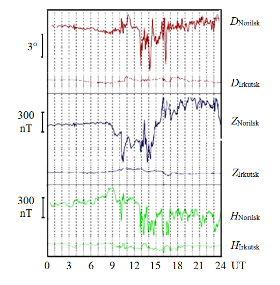
Variations of magnetic declination D, vertical Z and horizontal H components during the magnetic storm on March 22, 2026
The practical importance of choosing the right geomagnetic model is confirmed by economic indicators. A wellbore that goes beyond acceptable limits due to navigation errors leads either to the intersection of adjacent wells (loss of the well, costs for re-drilling a replacement well of \$0.5-2 million) or to the exit of the productive formation (a decrease in flow rate by 10-15%, loss of income of \$5-10 million over the entire productive period of the well). At a field with a typical number of horizontal wells (20-50 objects), annual losses from navigation errors without the use of special measures amount to \$100-150 million with a probability of two to three incidents per year [2].
Implementation of the CAMPUS-CA + DIF-1 + INTERMAGNET system requires an investment of \$10-17 million (including the development of local models, installation of observatories, and personnel training). The return on investment is \$28-54 million per year due to the elimination of navigation errors and increased flow rates thanks to precise positioning in productive formations. Thus, the return on investment is 165-540% per year, and full payback is achieved in 2-7 months. This demonstrates high economic feasibility of deploying the proposed system [17].
The strategic importance of developing local geomagnetic models for the Russian Federation is determined by the need to ensure technological independence in the critical field of oil and gas geophysics. Given the aforementioned cessation of access to foreign models, the development and implementation of domestic models (CAMPUS, DIF-1) and monitoring systems (INTERMAGNET) have become critically important. Russian models not only address the current challenge of import substitution but also surpass Western counterparts in accuracy and adaptability to local conditions[21]. This creates conditions for the development of export services in the field of geomagnetic modeling for other countries with Arctic deposits (Canada, Norway, Greenland) and also increases the investment attractiveness of Russian Arctic projects due to the proven possibility of safe drilling in conditions of high well density.
National geomagnetic models CAMPUS and DIF-1
The creation of the Earth’s main magnetic field model was initially carried out by the N.V.Pushkov Institute of Terrestrial Magnetism, Ionosphere, and Radio Wave Propagation (IZMIRAN), the leading institute for terrestrial magnetism. However, the transition to digital techno-logies and the launch of low-orbit satellites for magnetic field measurements led to a reassessment of these approaches. In 2022, the Geophysical Center of the RAS began work on adapting scientific results in modeling the Earth’s main magnetic field to the requirements of the oil and gas sector and the ISCWSA industry standard. Data from all satellite magnetometer missions [21] (CryoSat-2 [22-24], Ørsted [25, 26], CHAMP [27], Swarm [28, 29]) were collected. Next, using the ground-based observatory measurements and historical aeromagnetic data [30, 31], the CAMPUS model was created. The series of CAMPUS magnetic models (GC RAS) includes the model for the main magnetic field (CAMPUS-C) and for the lithospheric/anomalous field (CAMPUS-A). The complete model, designated as CAMPUS-CA, has a maximum resolution of 1050 spherical harmonics, providing spatial resolution ~38km.
The main field model is based on the IGRF-14 candidate model [21], prepared in the Geophysical Center of the RAS in 2024. The candidate model has passed all verification stages by the IGRF working group and was used to calculate the coefficients of the final international model for 2025-2030.
In 2022, the Trofimuk Institute of Petroleum Geology and Geophysics SB RAS developed the DIF-1 model (an analogue of the international IFR-1 model), which has been successfully used for three years at a northern field with a dense well grid for directional and horizontal drilling. The DIF-1 model is developed individually for a specific field based on available maps of anomalous magnetic fields or specially conducted aeromagnetic surveys. Interpretation of this data on the distribution of magnetic induction vector modulus anomalies, using other geological and geophysical information, makes it possible to reconstruct the distribution of magnetic properties of rocks in the Earth’s crust in the field area and, in the next step, calculate the spatial distribution of D, I, F magnetic field components. This allows for the construction of a detailed 3D geomagnetic model of the upper crust in the deposit area, including data on the main field and its secular variations, achieving a spatial resolution of a few kilometers. The advantage of the DIF-1 model is its high spatial resolution and high accuracy in determining magnetic field components: the determination errors for the D, I and F components’ absolute values are 0.1°, 0.05°, and 50nT, respectively. Conducting annual repeat observations of magnetic field component absolute values allows for annual model adjustments by taking into account the secular variation. The DIF-1 model is currently being developed for three more Arctic hydrocarbon fields.
In parallel, IZMIRAN is developing models with a decomposition degree of up to 790 harmonics (category HRGM), and its St. Petersburg branch, together with oil and gas companies, is conducting research on the construction of local IFR-1 models [32].
Physical principles of magnetic field modeling and their application in inclinometry in the Arctic
The magnetic field measured at the Earth’s surface includes several virtually independent signal sources:
where Bm(r,t) is the core (main) field; A(r) is the field of lithospheric sources; D(r,t) is the field from magnetosphere and ionosphere currents; e(t) is the measurement error.
The lithospheric source field is included as time-independent, since variations in the lithospheric field occur on geological time scales. The remaining components are time-dependent and require the construction of mathematical models that describe the temporal and spatial variability of the Earth’s magnetic field. The complexity of modeling the field sources varies significantly: low-orbit satellite observations have simplified the construction of main field models [33], and the global anomaly maps made it possible to construct a spherical decomposition of the lithospheric field. Modeling external fields is a daunting task. Moreover, while the mid-latitude ionospheric field is quite successfully approximated by spherical models based on satellite data [34], in practice it is impossible to predict high-latitude substorm disturbances since they are associated with non-stationary processes in the magnetosphere tail.
When horizontal drilling in the Arctic, it is critical to consider the D(r,t) component, as geomagnetic disturbances at high latitudes reach amplitudes of 1000-3000 nT and more, which exceeds the signal of the horizontal component of the magnetic field itself [35].
The main field is modeled using spherical harmonic analysis, first proposed by Gauss. The internal source field is represented as a gradient of a scalar potential V:
In order to calculate V, a series expansion in spherical functions through associated Legendre polynomials is used:
where a is the mean Earth’s radius (6371.2 km); gnm and hnm are the Gaussian coefficients of expansion; and r, θ, φ are the distance from the center, colatitude (a complementary angle to 90°), and longitude.
In this case, the spatial resolution of the model can be estimated through the minimum wavelength of the spherical expansion
where k is the maximum power of expansion.
In Table 4, information is given for the main sources of the Earth’s magnetic field and their time scales during inclinometry in the Arctic.
Table 4
The main sources of the Earth’s magnetic field and their time scales
|
Source |
Magnitude, nT |
Alternation period |
Description |
|
Internal |
|||
|
Core (main field) |
~50,000 |
Years |
Spherical expansion, IGRF/WMM models |
|
Lithosphere (anomalies) |
100-1000 |
Centuries |
Anomalous field maps, HRGM model |
|
External |
|||
|
High-latitude effects |
>1000 |
Hours to days |
Auroral substorms, unpredictable |
|
Mid-latitude effects |
10-100 |
Days |
Ionospheric field, approximated by models |
*Saltus R., Alken P., Balmes A. et al. Magnetic Maps and Models for Alternative Navigation. 2023 IEEE/ION Position, Location and Navigation Symposium (PLANS), 24-27 April 2023, Monterey, CA, USA. IEEE, 2023, p.805-813. DOI:10.1109/PLANS53410.2023.10140025
Modern high-resolution models such as CAMPUS-CA and BGGM provide a spatial resolution of 28-38 km, which is sufficient to account for regional anomalies but insufficient to identify local effects within a field. For this reason, critical horizontal drilling in the Arctic requires the use of models such as IFR-1 and DIF-1, with a spatial resolution of the first kilometers [36].
Ensuring the accuracy of the developed models and their prompt updating requires continuous observatory observations across the Russian network, allowing for the use of up-to-date data for the timely accounting of geomagnetic variations generated by processes in the Earth’s external envelopes (ionosphere, magnetosphere). Strong magnetic field disturbances in northern latitudes lead to azimuth measurement errors of more than 2° using borehole inclinometers due to differences in relatively quiet magnetic field parameters.
In horizontal drilling conditions, such azimuth changes in a dense well network are unacceptable and can lead to the intersection of adjacent wells. The observatory’s critical importance arises when drilling through well sections that require extremely precise positioning (reservoir entry, horizontal section, target zone). Therefore, it is necessary to deploy full-scale geomagnetic observatories in the vicinity of large oil and gas fields in the Far North, in addition to existing ones, as well as to continuously develop national high-resolution mathematical models.
History of the development of the Russian INTERMAGNET network
The gap in domestic instrumentation in the 1990s and a lack of resources led to a significant degradation of the Russian magnetic observatory network. The first Russian observatory (Irkutsk, IRT) joined the international INTERMAGNET network only in 1998, seven years after the network’s founding. Further restoration took place in the early 2000s with the support of international institutes, bringing the observatories of Borok (BOX), Novosibirsk (NVS), Yakutsk (YAK), Magadan (MGD), Paratunka (PET), and Arti (ARS) up to INTERMAGNET standards.
Significant changes occurred in 2011, when the Russian segment of the INTERMAGNET network was established at the Geophysical Center of the RAS. Since then, the Geophysical Center of the RAS has installed world-class equipment in five observatories, ensuring their compliance with international standards.
Currently, there are 12 magnetic observatories operating in Russia, including Klimovskaya (KLI) and Mikhnevo (MHV). Observatory-class measurements in the polar regions are carried out at the White Sea (WSE, Republic of Karelia) and Cape Schmidt (CPS, Chukotka Autonomous Okrug) observatories. All data are collected at the Shared Research Facility “Analytical Geomagnetic Data Center” of the Geophysical Center of the RAS, the center of the Russian INTERMAGNET segment.
Recently, the Samoylovsky Island (Sakha Republic) and Sabetta (Yamal Peninsula) observatories have been actively developed by the GC RAS and the IPGG SB RAS. However, the current coverage of the Arctic with geomagnetic observatories is insufficient to provide data for all Russian northern fields.
Requirements for observatories and recommendations for their placement in order to support horizontal drilling
The main challenges in developing high-precision observation sites in the Arctic are related to the region’s inaccessibility, the lack of necessary infrastructure, and the need for constant personnel presence, which translates into high operating costs. For the Yamal LNG project, annual costs for magnetic model corrections are estimated at \$200,000-\$500,000. The cost of a single fully functional observatory is at least 100 million rubles.
During horizontal drilling, effective development of geomagnetic models requires the establishment of a network of secular variation stations for regular observations at least annually. The need for such a network follows from an analysis of the geomagnetic observation situation in Russia, particularly in Siberia and the Far East. Research shows that due to the sparse network of ground-based geomagnetic observations in these regions, current models, which rely primarily on satellite data, do not provide the necessary accuracy in determining geomagnetic field components.
Optimal measurement correction quality during horizontal drilling is achieved at an observatory distance of no more than 200 km from the work site. This radius ensures proper interpretation of local magnetic anomalies and variations.
It is recommended that at least five specialized geomagnetic observatories be located in close proximity to the main Arctic oil and gas fields, which will ensure:
- continuous updating of regional models in real time;
- integration with existing monitoring systems;
- increase in the navigation data relevance up to ±0.5-1.0°;
- reducing the risk of emergency situations by 15-20%.
Analysis of spatial and temporal changes in the Arctic geomagnetic field for horizontal drilling
Analysis of features and values of changes of the magnetic field components (declination D, inclination I, total magnetic field magnitude F) in the northern Russian regions shows that:
- The magnetic inclination I and the field vector magnitude F experience relatively small and slow changes over the past 10-15 years in the northern regions of Siberia and the Arctic, whereas the magnetic declination D experiences much more intense spatial and temporal changes in these areas.
- A more rapid increase in absolute magnetic declination values is seen, especially since 2010.
- Abrupt jumps in annual changes in the model secular variation D every 5 years are due to the replacement of the IGRF models in these years and do not reflect the actual changes.
- Even high-resolution models (WMMHR) give errors in determining the magnetic declination D absolute value up to 0.8° in the Arctic areas, which emphasizes the need to develop and use high-precision local models.
These data indicate a critical need to develop dense repeat station networks [35] in order to register secular variation with the accuracy required for the development of HRGM and IFR models. In this context, IFR-1 level models, such as DIF-1, are of particular importance, the development of which is accompanied by direct high-precision measurements of the D, I and F components in the vicinity of a particular field.
Results of the application of high-precision inclinometry methods in the Arctic
The use of geomagnetic correction methods in horizontal drilling in the Far North has shown significant results at several fields [32, 37].
The successful implementation of the DIF-1 model at a field in Northern Siberia has stimulated the development of similar models for three more large fields in the Arctic zone of the Russian Federation. Annual model adjustments are made based on repeated absolute measurements of magnetic field components at control points.
The CAMPUS-CA model (GC RAS) is being tested and adapted at a number of fields, including those located in the Arctic zone of the Russian Federation. At Arctic fields, the deployment of specialized observatories has led to increased horizontal drilling efficiency due to more precise borehole positioning in target formations, which has increased the length of the productive section of the well and, consequently, the flow rate [38, 39]. The use of continuous high-frequency magnetic field monitoring with minute-by-minute updates made it possible to continue the process of product extraction during geomagnetic disturbances with a change rate of more than 10nT/min [40].
Conclusion
In the framework of the research, the geomagnetic models CAMPUS-C, CAMPUS-A, CAMPUS-CA and DIF-1 have been created. The CAMPUS-CA model is of HRGM class and has been built using CryoSat-2, Ørsted, CHAMP and Swarm satellite data; the expansion degree is 38 (1050 Gaussian coefficients); the model has been updated to 2024 and extrapolated to 2025-2030. The DIF-1 model complies with the IFR-1 class with an accuracy of D=±0.1°, I=±0.05°, F=±50nT.
Development and implementation of the CAMPUS-CA (GC RAS) and the DIF-1 (IPGG SB RAS) Earth’s magnetic field models supported by a network of geomagnetic observatories are a key factor in increasing the accuracy of inclinometry during drilling of oil and gas wells in the Arctic zone of the Russian Federation, especially during horizontal drilling in conditions of a dense well grid. In the absence of foreign supplies, geomagnetic field data, and the high instability of the magnetic field in the Far North, the use of Russian models fully satisfies the fuel and energy complex’s stringent requirements for the accuracy of geomagnetic data during horizontal drilling.
Expected practical results include:
- Improving the accuracy of inclinometry to 67-85% (reducing the error in determining the azimuth during horizontal drilling from ±2-3 to ±0.5-1.0°).
- Reducing the risk of emergency situations to 15-20% due to more precise well positioning [32].
- Increased oil recovery by 10-15% due to precise placement of horizontal sections of the well trajectory in productive formations.
- Increasing the efficiency of developing low-permeability reservoirs with an oil recovery factor of up to 40% or more [41].
- Reducing the environmental impact on the Arctic zone by reducing the number of vertical wells and the area of well pads by 30-40% [2].
- Increasing Russia’s technological independence in the field of geomagnetic support for oil and gas horizontal drilling projects [42].
For the further development of high-precision geomagnetic observations and magnetic field models it is recommended:
- to deploy at least five specialized geomagnetic observatories in close proximity to the main Arctic fields;
- to organize a network of repeat stations (at least 10-15 points) for monitoring the magnetic field secular variation;
- to ensure annual updating of CAMPUS-CA models and development of local DIF-1 models for each major field;
- to integrate data from Russian observatories into the Analytical Geomagnetic Data Center of the GC RAS with a minute-by-minute frequency;
- to organize the training of specialists to service observatories and interpret geomagnetic data when solving horizontal drilling problems;
- to include the requirements for the use of high-precision geomagnetic models in the technological regulations for drilling horizontal wells at all Arctic fields.
Thus, the implementation of an integrated geomagnetic monitoring system and high-precision models of the Earth’s magnetic field forms a sustainable technological base for the successful and safe development of Russia’s oil and gas potential in the Arctic and is of strategic importance for national security and economic development.
References
- Melnikov V.P., Osipov V.I., Brushkov A.V. et al. Decreased Stability of the Infrastructure of Russia’s Fuel and Energy Complex in the Arctic Because of the Increased Annual Average Temperature of the Surface Layer of the Cryolithozone. Herald of the Russian Academy of Sciences. 2022. Vol. 92. N 2, p. 115-125. DOI: 10.1134/S1019331622020083
- Zhdaneev O.V., Frolov K.N. Technological and institutional priorities of the oil and gas complex of the Russian Federation in the term of the world energy transition. International Journal of Hydrogen Energy. 2024. Vol. 58, p. 1418-1428. DOI: 10.1016/j.ijhydene.2024.01.285
- Novak A. Russian Fuel and Energy Complex 2022: Challenges, Results and Prospects. Energy Policy. 2023. № 2 (180), p. 4-11 (in Russian). DOI: 10.46920/2409-5516_2023_2180_4
- Rylance M., Aliyev S.A., Makarov A. et al. Paradigm Shift: Pad Optimization for a Potential Tight-Gas Development in Russia. SPE Russian Petroleum Technology Conference, 26-29 October 2020. OnePetro, 2020. N SPE-201989-MS. DOI: 10.2118/201989-MS
- El Sabeh K., Gaurina-Međimurec N., Mijić P. et al. Extended-Reach Drilling (ERD) – The Main Problems and Current Achievements. Applied Sciences. 2023. Vol. 13. Iss. 7. N 4112. DOI: 10.3390/app13074112
- Gupta V. P., Yeap A.H., Fischer K.M. et al. Expanding the Extended Reach Envelope at Chayvo Field, Sakhalin Island. IADC/SPE Drilling Conference and Exhibition, 4-6 March 2014, Fort Worth, TX, USA. OnePetro, 2014. N SPE-168055-MS. DOI: 10.2118/168055-MS
- Soloviev A.A., Sidorov R.V., Oshchenko A.A., Zaitsev A.N. On the Need for Accurate Monitoring of the Geomagnetic Field during Directional Drilling in the Russian Arctic. Izvestiya, Physics of the Solid Earth. 2022. Vol. 58. N 3, p. 420-434. DOI: 10.1134/S1069351322020124
- Onovughe E., Otobong T. Geomagnetic Referencing Techniques as Vital Directional Reference in Hydrocarbon Drilling. Journal of Multidisciplinary Engineering Science Studies. 2016. Vol. 2. Iss. 8, p. 836-841.
- Gvishiani A.D., Lukianova R.Yu. Estimating the Influence of Geomagnetic Disturbances on the Trajectory of the Directional Drilling of Deep Wells in the Arctic Region. Izvestiya, Physics of the Solid Earth. 2018. Vol. 54. N 4, p. 554-564. DOI: 10.1134/S1069351318040055
- Livermore P.W., Finlay C.C., Bayliff M. Recent north magnetic pole acceleration towards Siberia caused by flux lobe elongation. Nature Geoscience. 2020. Vol. 13. Iss. 5, p. 387-391. DOI: 10.1038/s41561-020-0570-9
- Ziehm T., Pare A., Willerth M. et al. Eliminating Drilling and Surveying Delays from Solar Storms with a Deployed Magnetic Observatory and Modern Workflow. SPE Annual Technical Conference and Exhibition, 20-22 October 2025, Houston, TX, USA. OnePetro, 2025. N SPE-228045-MS. DOI: 10.2118/228045-MS
- Ledroz A.G., Weston J.L. Patent N US 11041376 B2. Gyro-Magnetic Wellbore Surveying. Publ. 22.06.2021.
- Zhdaneev О.V., Zaytsev А.V., Prodan Т.Т. Possibilities for creating Russian high-tech bottomhole assembly. Journal of Mining Institute. 2021. Vol. 252, p. 872-884. DOI: 10.31897/PMI.2021.6.9
- Zhdaneev O.V., Zaitsev A.V., Lobankov V.M. Metrological support for the logging while drilling and wireline equipment. Journal of Mining Institute. 2020. Vol. 246, p. 667-677. DOI: 10.31897/PMI.2020.6.9
- Khomutov S.Yu. Problems of Processing of Raw Data from Magnetic Observatories: Will Modern Mathematical Technologies Help? Russian Journal of Earth Sciences. 2025. Vol. 25. N 2. N ES2022. DOI: 10.2205/2025ES000994
- Califf S., Nair M., Weimer D. et al. Assessment of the Weimer Geomagnetic Perturbation Model for High-Latitude Positioning and Navigation. Space Weather. 2024. Vol. 22. Iss. 10. N e2024SW004005. DOI: 10.1029/2024SW004005
- Zhdaneev O.V., Ovsyannikov I.R. From import substitution to technological leadership: how local content policy accelerates the development of the oil and gas industry. Journal of Mining Institute. 2025. Vol. 274, p. 177-194.
- Soloviev A.A., Sidorov R.V., Oshchenko A.A., Zaitsev A.N. On the Need for Accurate Monitoring of the Geomagnetic Field during Directional Drilling in the Russian Arctic. Izvestiya, Physics of the Solid Earth. 2022. Vol. 58. N 3, p. 420-434. DOI: 10.1134/S1069351322020124
- Ruifeng Yu, Binbin Diao, Deli Gao. Calculation for Wellbore Trajectory Measurement Error Incorporating Magnetic Azimuth Correction. Petroleum Drilling Techniques. 2023. Vol. 51. N 6, p. 25-31. DOI: 10.11911/syztjs.2023056
- Momot F., Humbled F., Garbers M. et al. First Onsite Automatic Geomagnetic Observatory Improves Well-Bore Positioning. International Petroleum Technology Conference, 26-28 March 2019, Beijing, China. OnePetro, 2019. N IPTC-19395-MS. DOI: 10.2523/IPTC-19395-MS
- Firsov I., Kudin D., Soloviev A. et al. GCRAS candidate field models for IGRF-14. Earth, Planets and Space. 2026. Vol. 78. N 9. DOI: 10.1186/s40623-025-02318-2
- Hammer M.D., Finlay C.C., Olsen N. Applications for CryoSat-2 satellite magnetic data in studies of Earth’s core field variations. Earth, Planets and Space. 2021. Vol. 73. N 73. DOI: 10.1186/s40623-021-01365-9
- Park J., Stolle C., Yamazaki Y. et al. Diagnosing low-/mid-latitude ionospheric currents using platform magnetometers: CryoSat-2 and GRACE-FO. Earth, Planets and Space. 2020. Vol. 72. N 162. DOI: 10.1186/s40623-020-01274-3
- Olsen N., Albini G., Bouffard J. et al. Magnetic observations from CryoSat-2: calibration and processing of satellite platform magnetometer data. Earth, Planets and Space. 2020. Vol. 72. N 48. DOI: 10.1186/s40623-020-01171-9
- Neubert T., Mandea M., Hulot G. et al. Ørsted satellite captures high-precision geomagnetic field data. Eos, Transactions American Geophysical Union. 2001. Vol. 82. Iss. 7, p. 81-88. DOI: 10.1029/01EO00043
- Nielsen O.V., Petersen J.R., Primdahl F. et al. Development, construction and analysis of the “OErsted” fluxgate magnetometer. Measurement Science and Technology. 1995. Vol. 6. N 8, p. 1099-1115. DOI: 10.1088/0957-0233/6/8/004
- Reigber C., Lühr H., Grunwaldt L. et al. CHAMP Mission 5 Years in Orbit. Observation of the Earth System from Space. Springer, 2006, p. 3-15. DOI: 10.1007/3-540-29522-4_1
- Olsen N., Finlay C.C., Kotsiaros S., Tøffner-Clausen L. A model of Earth’s magnetic field derived from 2 years of Swarm satellite constellation data. Earth, Planets and Space. 2016. Vol. 68. N 124. DOI: 10.1186/s40623-016-0488-z
- Yi Jiang, Holme R., Yong Jiang. Investigation of the consistency of Swarm data and CHAOS-6 towards crustal magnetic field studies in China. Applied Geophysics. 2023. Vol. 20. Iss. 4, p. 422-431. DOI: 10.1007/s11770-021-0968-1
- Meyer B., Chulliat A., Saltus R. Derivation and Error Analysis of the Earth Magnetic Anomaly Grid at 2 arc min Resolution Version 3 (EMAG2v3). Geochemistry, Geophysics, Geosystems. 2017. Vol. 18. Iss. 12, p. 4522-4537. DOI: 10.1002/2017GC007280
- Lesur V., Hamoudi M., Yujin Choi et al. Building the second version of the World Digital Magnetic Anomaly Map (WDMAM). Earth, Planets and Space. 2016. Vol. 68. N 27. DOI: 10.1186/s40623-016-0404-6
- Bukhtoyarov B.N., Starikova O.R., Petrov V.G. et al. Geomagnetic data for directional drilling and well positioning. Mine Surveying and Subsurface Use. 2025. Vol. 25. N 4, p. 71-82 (in Russian). DOI: 10.56195/20793332-2025-25-4-71-82
- Chulliat A., Vigneron P., Thébault E. et al. Swarm SCARF Dedicated Ionospheric Field Inversion chain. Earth, Planets and Space. 2013. Vol. 65. Iss. 11, p. 1271-1283. DOI: 10.5047/eps.2013.08.006
- Sado P., Clausen L.B.N., Miloch W.J., Nickisch H. Substorm Onset Prediction Using Machine Learning Classified Auroral Images. Space Weather. 2023. Vol. 21. Iss. 2. N e2022SW003300. DOI: 10.1029/2022SW003300
- Kuleshov D.A., Dyadkov P.G., Plotkin V.V. Correction for Geomagnetic Secular Variation Effects: A New Method (Case Study of the Altai Geodynamic Network). Russian Geology and Geophysics. 2021. Vol. 62. N 2, p. 255-262. DOI: 10.2113/RGG20194056
- Califf S., Nair M., Weimer D. et al. Assessment of the Weimer Geomagnetic Perturbation Model for High-Latitude Positioning and Navigation. Space Weather. 2024. Vol. 22. Iss. 10. N e2024SW004005. DOI: 10.1029/2024SW004005
- Bukhtoyarov B.N., Starikova O.R., Petrov V.G. et al. Geomagnetic data for directional drilling and well positioning. Mine Surveying and Subsurface Use. 2025. Vol. 25. N 4, p. 71-82 (in Russian). DOI: 10.56195/20793332-2025-25-4-71-82
- Ziehm T., Pare A., Willerth M. et al. Eliminating Drilling and Surveying Delays from Solar Storms with a Deployed Magnetic Observatory and Modern Workflow. SPE Annual Technical Conference and Exhibition, 20-22 October 2025, Houston, TX, USA. OnePetro, 2025. N SPE-228045-MS. DOI: 10.2118/228045-MS
- Beggan C.D., Clarke E., Knight P. et al. Assessing the Absolute and Relative Accuracy of Magnetic Variometers Compared to Observatory Data for IFR2. SPE/IADC International Drilling Conference and Exhibition, 4-6 March 2025, Stavanger, Norway. OnePetro, 2025. N SPE-223681-MS. DOI: 10.2118/223681-MS
- Marr T., Schiermeier P. Application of MWD Survey Corrections in Real Time. SPE/IADC Middle East Drilling Technology Conference and Exhibition, 26-28 January 2016, Abu Dhabi, UAE. OnePetro, 2016. N SPE-178172-MS. DOI: 10.2118/178172-MS
- Zhdaneev O.V. Technological sovereignty of the Russian Federation fuel and energy complex. Journal of Mining Institute. 2022. Vol. 258, p. 1061-1078. DOI: 10.31897/PMI.2022.107
- Soloviev A.A. Geomagnetic support for directional drilling. Herald of the Russian Academy of Sciences. 2024. Vol. 94. N 10, p. 885-891 (in Russian). DOI: 10.31857/S0869587324100023