
Improving the method for assessment of bending stresses in the wall of an underground pipeline
- 1 — Ph.D., Dr.Sci. Rector Ukhta State Technical University ▪ Orcid
- 2 — Postgraduate Student Saint Petersburg Mining University ▪ Orcid

Abstract
Brief information about modern methods for determining the bending stresses of the extended sections of underground main pipelines without access to the pipeline generatrix is given. The necessity of modernizing methods based on determining the configuration of the pipeline axis from the soil surface with subsequent calculation of bending stresses based on the obtained data is substantiated. A mathematical model that allows to calculate the optimal parameters for surveying the axis of the pipeline from the soil surface for a pipeline of arbitrary configuration and depth, when planning a study, is proposed. Bench tests of the BITA-1 pipeline finder were carried out to determine the error in measuring the depth of the pipeline axis. It is proved that the deviations of the pipeline finder data relative to the true values in narrow depth intervals follow a normal distribution and do not change their sign. The confidence intervals of the error in determining the depth of the pipeline axis for the BITA-1 device are presented.
None
Introduction
Hydrocarbons play an important role in the modern fuel and energy balance, being an integral part of modern industry [1-3]. With the help of main pipelines, a constant and uninterrupted supply of hydrocarbons from production sites to the consumer is possible [4, 5]. Therefore, methods and technologies that allow for reliable and proper operation of main pipelines took important places.
Accidents at existing oil and gas pipelines are associated with enormous damage to the environment and huge material damage [6-8], caused by loss of pumped product and failures in delivery times, as well as shutdown of the entire system for unscheduled repairs [9-10].
The most difficult to predict types of accidents include the ones that associated with the impact of external force factors on the pipeline, which lead to the formation of an abnormal bend in the pipeline [11-13]. As a rule, when designing a pipeline, the strength of the pipeline is laid down in the calculation of the wall thickness of the pipes [14-16], which takes into account the effect of permanent loads [17]. However, this calculation does not take into account the possibility of other loads and impacts affecting the pipeline that occur during the operation period, since their accounting at an arbitrary point in time cannot be mathematically described [18-20]. The actual operating conditions of the main gas and oil pipelines are different, which is confirmed by a large number of correction factors introduced into the strength calculations.
Despite the existence of a large number of methods for assessing the stress-strain state of steel structures [21, 22], most of them are hardly applicable to main pipelines due to the difficulty of determining mechanical stresses in the extended sections of underground pipelines, and the frequency of in-line diagnostics does not allow it to be classified as a system for continuous monitoring of the technical condition of the pipeline. Therefore, it is necessary to assess the actual state of an underground gas and oil pipeline during the entire period of its operation at an arbitrary point in time in accordance with changing engineering and geological conditions. Under these conditions, methods that allow assessing the technical condition at an arbitrary point in time are of particular relevance.
Modern methods and problems of determining the technical condition of extended sections of underground pipelines
The technical condition of the pipeline is usually understood as a combination of factors affecting the reliable and trouble-free operation of the pipeline. One of the most important parameters that determine the technical condition of the pipeline is the stress-strain state (SSS) of the metal of the pipeline walls, which also depends on a large number of loads and influences that affect the pipeline. Among the main sources of the stress state, bending stresses can be distinguished [11, 14, 18]. Let us consider the main methods for determining SSS in sections of underground pipelines that do not require constant access to the pipeline generatrix.
Methods based on measuring the physical fields of the pipeline have proven themselves well: magnetometric [16, 23], using smart inserts [24, 25], ultrasonic [25]. With information about the initial stress state, this family of methods is the most accurate, and some methods [23, 26] that show a high accuracy of determining the SSS without information about the initial stress state. The most significant disadvantage of these methods is the need for access to the pipeline generatrix in order to install specialized equipment. In addition, their application implies the presence of a priori knowledge about the sections of the pipeline, in which additional bending stresses may appear, however, the distribution of these sections along the length of the pipeline is not constant during its operation.
Stress-strain state of the pipeline calculation is possible according to regulatory standards if there is information on the values of bending stresses acting in the controlled areas [16, 27]. Recently, much attention has been paid to methods based on the use of fiber-optic sensors, which allow remotely assessing the bending of the pipeline at an arbitrary point in time during its operation [19, 28, 29]. For example, this system is used to monitor especially dangerous sections of the Sakhalin – Khabarovsk – Vladivostok gas pipeline with a diameter of 1220 mm. The use of this method allows you to quickly establish the development of off-design bends in sections of underground main pipelines, including those lying at the boundaries of active tectonic faults [19, 29]. During the operation of these systems, problems arose – damage to the fiber-optic deformation sensors by the geological environment, which entailed failure and false positive responses of the system. For the effective use of these methods, it is necessary to develop auxiliary methods that will confirm (or refute) the presence of off-design bends in controlled areas.
This can be a method for determining bending stresses in the wall of an underground main pipeline based on data on the configuration of the axis of the pipeline, the main advantages of which are low cost, simplicity and the possibility of using it for monitoring extended sections of main pipelines. The wide application of this method is limited by a poorly developed scientific and technical base.
A number of research papers offer various options for estimating the bending stresses based on pipeline axis survey data. In the works [30, 31] it is recommended to use polynomials of high degree to approximate the axis of the pipeline, in the works [25, 32] the authors propose to use the chord method. In addition, there are VRD 39-1.10-026-2001 standards and VNIIST R-352-79 recommendations that suggest using a fixed step when surveying the pipeline axis. These approaches rely on assumptions that are not always met in practice [12, 14, 28]. For example, when using the chord method, a fixed distance between measurement points is required, and in calculations, according to this method, the maximum depth in the measurement area is taken as the actual depth of the pipeline axis at all measurement points. It is also assumed that the error of the devices used to determine the depth of the pipeline axis does not change during the survey.
The main problems and opportunities for modernizing this technique are described in the work [33]. The main limitation of all existing methods is the use of the maximum depth in the control area when performing calculations, as well as the fixed error of the trace finder in the entire control area. Based on literary sources [34, 35], it can be said that when crossing natural and artificial obstacles, sections of an underground pipeline can be buried by more than 10 m, while at 100 m from this crossing the depth may not reach 2-3 m. The error of the device at different measurement points can also vary significantly depending on the shooting conditions (humidity, temperature, etc.). All boundary cases are pointing to the need of refining the techniques [25, 31, 32] to assess bending stresses for various design parameters of both the pipeline itself and pipe laying conditions, as well as the equipment used and the location of the survey.
Research methodology
Refinement of a mathematical model similar to that described in the source [33], is associated with the need to search for a large amount of data for the selection of regression coefficients. These data can be obtained by modeling the elastic bending of a pipeline section with fixed parameters. The work uses data similar to those used in the work [33], with the addition of several new input variables. A detailed diagram of the model is described in the materials [25, 32, 33].
The developed mathematical model is set by the following parameters:
where D – investigated pipeline diameter, m; hl, hr, hm, – depth of the pipeline axis at the left, right and central measurement points, m; Δl,Δr, Δm – error in measuring the depth of the pipeline axis at the left, right and central measurement points, %; L – step between the measurement points of the pipeline axis depth, m; σ – maximum error in determining bending stresses when using these parameters, MPa.
For the developed mathematical model (1), it is necessary to select regression coefficients that minimize a certain metric by which one can judge the quality of the developed model. The traditional quality metric of regression problems is the root mean square error of measurements, however, for this problem it will be difficult to interpret due to the large spread in the values of the predicted value (error in determining bending stresses). Therefore, it is customary to use the average absolute percentage error as the target metric, which shows in percentage how much the model forecast is not accurate on average. The average absolute percentage error is expressed in terms of the ratio
where yi, yˆi – the true value of the quantity and predicted by the model, respectively; ε – an arbitrary positive small value used to avoid division by zero.
The use of this metric makes it possible to take into account the same weights for errors on response values of any order, i.e. forecast value scale.
The values hl, hr, hm; Δl,Δr, Δm; L are continuous, so they can be added to the regression model in their original form. The value of the pipeline diameter is a discrete value; in relation to optimization problems, these values are usually called ordinal, meaning that there is no possibility to compare them with each other, as it can be done with continuous ones. To this end, various approaches are used to encode ordinal variables; [36], in this work, the One Hot Encoding method was used – encoding with one “hot” variable [36]. The pipeline diameter is encoded as an n-dimensional vector, where n is the number of unique categories of a given feature. In our task, only main pipelines are considered, therefore, a number of investigated diameters include 1420, 1220, 1020, 820, 720, 520, 320, 220 mm.
Then the mathematical model will take 14 features as input, and output one feature equal to the error in the calculation of bending stresses when using these features:
where n – number of examples.
The optimization problem will look like this:
where X – matrix of input data presented in tabular form by column concatenation; l – the number of elements in the data sample.
Discussion and results
The solution of the optimization problem (2) implies the choice of not only the optimal values of the weights of the matrices W, but also their minimum size, since the size of the matrices W will significantly affect the algorithmic complexity of calculations on the devices where this mathematical model will be implemented. API [36] was used to search for coefficients, Adam [36, 37] was selected as the minimization method with default options. To speed up the
learning process, all integer variables supplied to the model input were normalized to bring their distributions to normal ones with zero mathematical expectation and unit variance. The final view of the nonlinear mathematical model of the pipeline diameter dependence, the error of the equipment used, the step between the measurement points and the depth of the pipeline axis on the maximum error in determining the bending stresses are described below:
where W1-4 – coefficient (weights) matrices are selected in the optimization process; b1-4 – the values of the offsets selected in the optimization process; – sigmoid function, applied element by element, equal to sigm (x)=1/(1+exp(-x)).
The sizes of the final matrices with coefficients obtained during the optimization process are presented in Table 1.
Table 1
Parameters of the developed mathematical model (3)
|
Parameter |
Matrix size |
Parameter |
Matrix size |
|
W1 |
(14, 15) |
b1 |
(15, 1) |
|
W2 |
(15, 20) |
b2 |
(20, 1) |
|
W3 |
(20, 15) |
b3 |
(15, 1) |
|
W4 |
(20, 1) |
b4 |
(1, 1) |
After optimization, MAPE = 0.67 %, so the average error between the true value of the error in determining the bending stresses and the value determined on the basis of the model (3) is quite small, and it is advisable to use this model for further research. To control the overfitting of the model for the data, the result is presented for a test sample, which was obtained by random sampling of 15 % of the original sample prepared for training. To control overfitting, L1, L2 regularizations were used.
Both the developed mathematical model (3) and the models of other researchers [25, 31, 32] suggest that the error value of the device, which measures the depth of the pipeline axis, does not exceed a certain constant value, which for modern route finders is about ±5 %. However, to obtain adequate results, it is also necessary that the deviations of the pipeline finder data from the error actual values during measurements should be of the same sign on the same depth, otherwise the bending stresses calculated on the basis of these data may either not correspond to reality or be not conservative with respect to true bending stresses.
Modern literary sources do not reflect information on the dispersion of the error of pipeline finders when measuring in narrow depth intervals, so we have a methodology that needs to be tested with the help of experimental studies. For these purposes, the errors of the BITA-1 type finder were determined for various values of the depth of the pipeline axis. Since the soils do not have a significant effect on the accuracy of the route finders [38], it was not the depth of the pipeline that was measured, but the distance between the axis of the pipeline and the receiver, which under these conditions is an assumption (Fig.1). The maximum passport error of the device is ±5 %.
The error in determining the depth of the pipeline axis by the pipeline finder (± 5 %) is indicated taking into account the effect of the most conservative set of factors on the device, while these factors may not be present on a real pipeline, which can increase the accuracy of the device.
An important factor in surveying the depth of an underground pipeline axis is also the obtained data dispersion. When surveying with a pipeline finder, it is assumed that at a fixed depth of the pipeline axis, deviations in determining the distances from the pipeline axis to the pipeline finder receiver (occurrence depth) will be of the same sign. For example, at a depth of 1-2 m, the device is mistaken in the range from 1 to 3 %.
The goals of the experimental study are to determine the confidence intervals of the device error in narrow depth intervals (by 1 m) and to confirm the hypothesis of homoscedasticity of the error variance in narrow depth intervals (by 1 m).
To achieve the goals, you need to do the following:
- fix the device data for the selected range of distances from the receiver of the device to the axis of the investigated pipeline;
- check the data obtained by the device and the true values measured with a tape measure;
- evaluate point statistics of device error;
- derive interval estimates of the device error at different distances from the receiver to the axis of the pipeline;
- draw conclusions based on the data received.
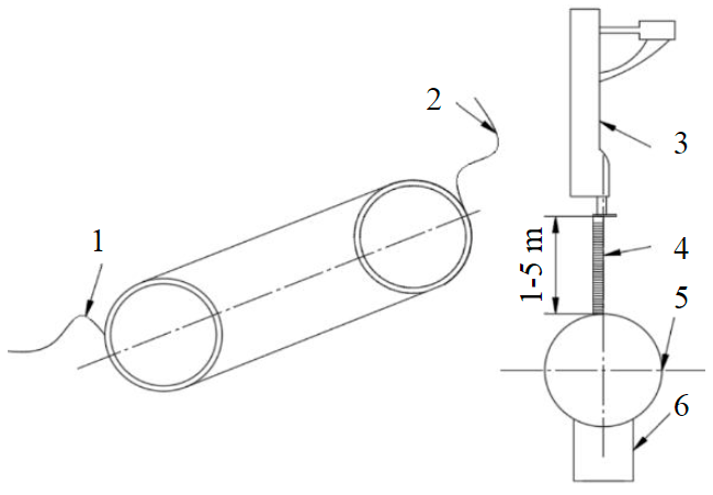
Fig.1. Measuring stand scheme 1 – connection to a current source; 2 – grounding; 3 – BITA-1 pipeline finder; 4 – tape measure; 5 – pipeline; 6 – pipeline support
For each distance from the pipeline axis to the receiver, eight measurements are made, each measurement consists of three, which are then averaged. Thus, for each value of the distance between the axis of the pipeline and the receiver, there are eight device measurements. Data obtained by measuring with a tape measure with an error of no more than ±0.45 mm/m are used as the true distance. Accurate installation of the device above the axis of the pipeline is guaranteed by means of determining the axis of the pipeline built into the BITA-1 device. During the measurements, a section of the pipeline with a diameter of 220 mm and a length of 35 m with an insulating bitumen coating was used (Fig.1). For the operation of the pipeline finders, it is necessary that an electric current flow through the body of the pipeline. On actually operating pipelines, the possibility of searching for the axis of the pipeline by route finders is ensured by its connection to cathodic protection stations. On the measuring bench, the current source is the generator included in the BITA-1 set, which is connected with clamps to the ends of the pipeline, the other end of the pipeline is grounded. Current frequency during measurements is 640 Hz, according to the recommendations of the source [38]. The interval between studied depths of one meter was adopted by experts in order to fix statistically significant differences based on the results of the work [25, 33].
An example of measurements results carried out in accordance with the described provisions is presented in Table 2. Measurements near connections to ground and a current source from a generator are associated with the occurrence of significant interference from induced current sources, which causes an additional measurement error. To level the error, the measurements on the experimental stand were made in the center of the pipeline.
Table 2
Measurement results at frequency of 640 Hz
|
Lact, m |
Lm1, m |
Lm2, m |
Lm, m |
Error, % |
|
1.1 |
1.090 |
1.090 |
1.100 |
–0.61 |
|
1.1 |
1.100 |
1.100 |
1.100 |
0.00 |
|
1.1 |
1.090 |
1.100 |
1.100 |
–0.30 |
|
1.1 |
1.100 |
1.100 |
1.080 |
–0.61 |
|
1.1 |
1.090 |
1.090 |
1.100 |
–0.61 |
|
1.1 |
1.080 |
1.100 |
1.100 |
–0.61 |
|
1.1 |
1.089 |
1.096 |
1.090 |
–0.77 |
|
1.1 |
1.090 |
1.086 |
1.099 |
–0.78 |
|
… |
… |
… |
… |
… |
|
5.1 |
5.140 |
5.120 |
5.130 |
0.59 |
|
5.1 |
5.190 |
5.150 |
5.160 |
1.31 |
|
5.1 |
5.150 |
5.140 |
5.170 |
1.05 |
|
5.1 |
5.180 |
5.180 |
5.180 |
1.57 |
|
5.1 |
5.180 |
5.200 |
5.180 |
1.70 |
|
5.1 |
5.240 |
5.200 |
5.200 |
2.22 |
|
5.1 |
5.190 |
5.150 |
5.170 |
1.37 |
|
5.1 |
5.150 |
5.140 |
5.170 |
1.05 |
The average value of the depth of occurrence set by the instrument is calculated by the formula:
where Lm – distance from the receiver to the axis of the cylindrical conductor (pipeline), m.
The average value of the instrument error in determining the depth is calculated by the formula:
where Lhiact – actual value of the depth of the pipeline axis, m.
Sample statistics of depth groups are given in Table 3. When processing the results of experimental studies, as a sample, the error in determining the depth of the pipeline axis, calculated as the average of three measurements (4), was used.
Table 3
Selected statistics by depth groups at a current frequency of 640 Hz
|
Parameter |
Depth of the axis h, m |
||||
|
1.1 |
2.1 |
3.1 |
4.1 |
5.1 |
|
|
Minimal errror Δmin, % |
–1.32 |
–1.27 |
1.51 |
0.41 |
0.59 |
|
Maximum error Δmax, % |
0 |
0.48 |
2.37 |
1.22 |
2.22 |
|
Avarage error Δhiavg% |
–0.552 |
–0.734 |
1.986 |
0.746 |
1.356 |
|
Sample standard deviation, % |
0.353 |
0.544 |
0.274 |
0.309 |
0.461 |
At small values of the axis depth (up to 2 m), the device shows lower depth values relative to the actual ones (Table 3). With an increase in the depth of occurrence, the device shows higher values of the occurrence depth of relative to the actual ones. When examining the occurrence depths on actual pipelines and the subsequent use of the data obtained to assess the level of bending stresses, it is necessary to determine the maximum values of the error in determining the depth of the pipeline axis, as well as the deviations dispersion in narrow intervals. We investigate the nature of the distribution using a non-parametric method for estimating the density of a random variable – a kernel density estimate (Fig.2) [34].
Error distributions are similar to normal ones (Fig.2), but each depth has its own parameters of the mean and standard deviation. The normal distribution has a number of good properties that can be used in practice. So, knowing the statistics of the normal distribution, you can build confidence intervals for the error when measuring at a certain depth and use the data obtained to calculate the bending stresses.
Let us estimate more strictly whether the error in measuring the depth of the pipeline axis with the BITA-1 device has a normal distribution. The most powerful criterion for a distribution to be normal is the Shapiro – Wilk test [35]. Shapiro – Wilk test statistics:
where s2 – sample dispersion; а – tabular coefficient.
The critical values of the W statistic are tabular. Let us estimate whether the distribution of sample data will correspond to the normal one using the Shapiro – Wilk test at the significance level of α = 0.95.
To automate the process, we will use the implementation of the Shapiro – Wilk criterion calculation, presented in the stats package of the Python programming language.
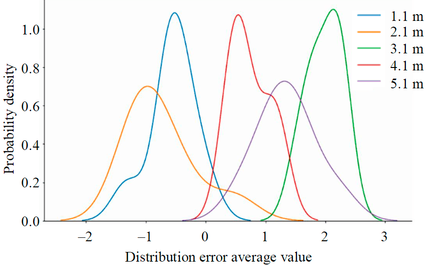
Fig.2. Kernel estimation of the distribution density in the study of the depths h
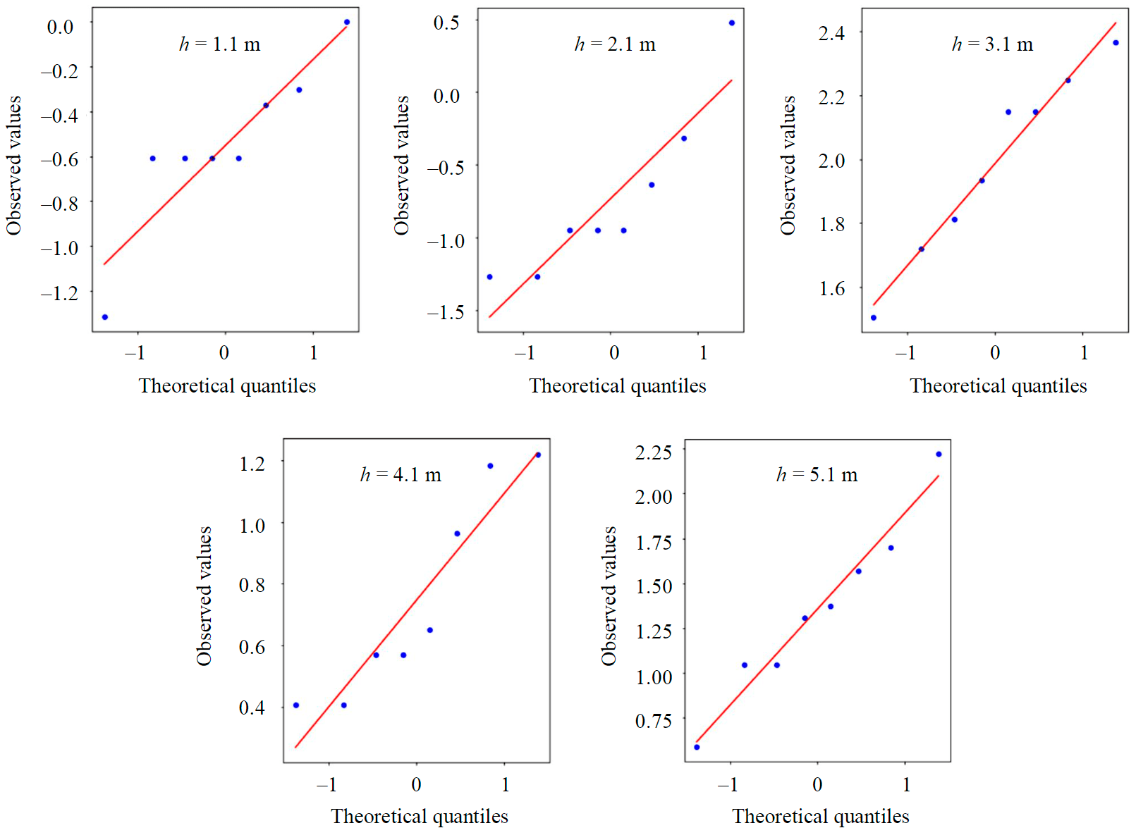
Fig.3. Distribution estimation with Q-Q plot
The p-value (at a significance level of 0.95) for the pipeline axis depth of 1.1 m is 0.036, which does not correspond to a normal distribution. Values corresponding to the normal distribution: 0.084 (depth 2.1 m); 0.975 (3.1 m); 0.637 (4.1 m); 0.968 (5.1 m).
At a depth of 1.1 m, the distribution of the error in measuring the depth of the axis of the pipeline is different from normal. Further, when constructing confidence intervals of measurement errors, it is planned to use T-statistics, one of the features of which is that it does not require a complete correspondence of the distribution to the normal one: it is enough for the distribution only visually corresponds to the normal [39]. One way to visually assess the normality of a distribution is the Q-Q plot (quantile-quantile plot).
The analysis of data on the Q-Q plot is based on a comparison of the theoretical quantiles of the normal distribution to the values distribution obtained from the experiments results in the sample. Let us use the Q-Q plot implementation from the stats package. Let us evaluate visually whether the sample data could be formulated by a normal distribution (Fig.3).
At a depth of 1.1 m (Fig.3), there is some discreteness around the average, which may indicate the adjustment of the equipment filters used. T-statistics allows you to build confidence intervals based on non-normal distributions if they are not strongly shifted [39], distribution of errors at a depth of 1.1 m satisfy the required conditions.
Since the dispersion of the general population is not known, 99 % of the confidence intervals of the average measurement error at each occurrence depth will be estimated using the Student's T-statistics of the distribution with degrees of freedom n – 1:
where X¯ – sample average; µ – population average; n – number of sample elements; S – unshifted sample standard deviation.
Then the confidence interval of the unknown average error in determining the depth of the pipeline axis m under the condition of the observed average X¯ will be equal to
where t – the required quantile of Student's distribution.
Confidence intervals for the average error in determining the depth of the pipeline axis based on Student's T-distribution: at h = 1.1 m confidence interval –0.9 ≤ µ ≤ –0.2; at h = 2.1 m interval –1.5 ≤ µ ≤ 0; at h = 3,1 m interval 1.6 ≤ µ ≤ 2.3; at h = 4.1 m interval 0.2 ≤ µ ≤ 1; at h = 5.1 m interval 0.7 ≤ µ ≤ 2.
Based on the results of calculating the BITA-1 pipeline finder error in determining the pipeline depth, it was found that in narrow depth intervals, the deviation of measurements relative to the true values does not change its sign, and the absolute value of the error does not exceed the passport values.
Thus, in order to calculate the bending stresses of an underground pipeline section based on the pipeline axis configuration data, it is necessary to calculate the required step between the measurement points using the mathematical model (3) and the methodology described in the article [33], to survey the configuration of the axis of the underground pipeline and, according to the obtained values using geometric positions [25, 32, 33], recalculate the obtained bending radii in the section into bending stresses.
Conclusion
A mathematical model has been improved for determining the optimal measurement step when surveying the depth of the underground pipeline axis from the soil surface for subsequent calculation of bending stresses in the pipeline wall based on the data obtained. The mathematical model makes it possible to take into account the variable error and the depth of the axis at each measurement point, as well as the design features of the investigated pipeline and laying conditions. The maximum error of the developed model on a delayed sample according to the MAPE metric = 0.67 %, according to the MAE metric = 3.5 MPa.
Based on the experimental studies of determination the error of the BITA-1 pipeline finder in a narrow depth interval (1 m each), it was found that the error dispersion in determining the depth of the pipeline axis is always of the same sign relative to the true depth, which will make it possible to make calculations with sufficient accuracy after surveying data. It is proved that the error of the device in a narrow depth interval obeys the normal distribution, or does not differ much from it. 99 % confidence intervals of the error in determining the depth of the pipeline axis in percent for the BITA-1 pipeline finder are calculated. It is shown that these error values never exceed the rating values of the device.
References
- Litvinenko V. The Role of Hydrocarbons in the Global Energy Agenda: The Focus on Liquefied Natural Gas. Resources. 2020. Vol. 9. Iss. 5. N 59. DOI: 10.3390/resources9050059
- Litvinenko V.S., Tsvetkov P.S., Dvoynikov M.V., Buslaev G.V. Barriers to implementation of hydrogen initiatives in the context of global energy sustainable development. Journal of Mining Institute. 2020. Vol. 244, p. 428-438. DOI: 10.31897/PMI.2020.4.5
- Dvoynikov M.V., Budovskaya M.E. Development of a hydrocarbon completion system for wells with low bottomhole temperatures for conditions of oil and gas fields in Eastern Siberia. Journal of Mining Institute. 2022. Vol. 253, p. 12-22. DOI: 10.31897/PMI.2022.4
- Fetisov V.G., Tcvetkov P.S., Müller J.M. Tariff Approach to Regulation of the European Gas Transportation System: Case of Nord Stream. Energy Reports. 2021. Vol. 7. N 6, p. 413-425. DOI: 10.1016/j.egyr.2021.08.023
- Zhengbing Li, Yongtu Liang, Weilong Ni et al. Pipesharing: economic-environmental benefits from transporting biofuels through multiproduct pipelines. Applied Energy. 2022. Vol. 311. N 18684. DOI: 10.1016/j.apenergy.2022.118684
- Biezma M.V., Andrés M.A., Agudo D., Briz E. Most fatal oil & gas pipeline accidents through history: A lessons learned approach. Engineering Failure Analysis. 2020. Vol. 110. N 104446. DOI: 10.1016/j.engfailanal.2020.104446
- Guoyun Shi, Weichao Yu, Kun Wang et al. Time-dependent economic risk analysis of the natural gas transmission pipeline system. Process Safety and Environmental Protection. 2021. Vol. 146, p. 432-440. DOI: 10.1016/j.psep.2020.09.006
- Islamov R.R., Fridlyand Ya.M., Aginey R.V. Retrospective analysis of failures causes at the main oil and gas pipelines, working in complicated engineering-geological conditions. Equipment and technologies for oil and gas complex. 2017. N 6, p. 80-87 (in Russian).
- Chio Lam, Wenxing Zhou. Statistical analyses of incidents on onshore gas transmission pipelines based on PHMSA database. International Journal of Pressure Vessels and Piping. 2016. Vol. 145, p. 29-40. DOI: 10.1016/j.ijpvp.2016.06.003
- Golyanov A.I., Golyanov A.A., Kutukov S.E. Review of main pipelines energy efficiency estimation methods. Problems of gathering, treatment and transportation of oil and oil products. 2017. N 4 (110), p. 156-170 (in Russian). DOI: 10.17122/ntj-oil-2017-4-156-170
- Ovchinnikov N.Т. Technical issues of applying the curvature radii in monitoring the pipeline conditions. Science & Technologies: Oil and Oil Products Pipeline Transportation. 2018. Vol. 8. N 3, p. 278-289 (in Russian). DOI: 10.28999/2541-9595-2018-8-3-278-289
- Askarov R.M., Valeev A.R., Islamov I.M., Tagirov M.B. Analysis of the effect of geodynamic zones crossing the main gas pipelines on their stress-strain state. Bulletin of the Tomsk Polytechnic University. Geo Assets Engineering. 2019. Vol. 330. N 11, p. 145-154. DOI: 10.18799/24131830/2019/11/2358
- Bakesheva A.T., Fetisov V.G., Pshenin V.V. A refined algorithm for leak location in gas pipelines with determination of quantitative parameters. International Journal of Engineering Research and Technology. 2019. Vol. 12. N 12, p. 2867-2869.
- Gumerov A.K., Silvestrov S.A. Development of estimation methods of allowable values of a pipeline elastic bending radius. Neftegazovoye delo. 2018. Vol. 16. N 4, p. 96-107 (in Russian). DOI: 10.17122/ngdelo-2018-4-96-107
- Sultanbekov R., Islamov Sh., Mardashov D. et al. Research of the influence of marine residual fuel composition on sedimentation due to incompatibility. Journal of Marine Science and Engineering. 2021. Vol. 9. N 1067. DOI: 10.3390/jmse9101067
- Krivokrysenko E.A., Popov G.G., Bolobov V.I., Nikulin V.E. Use of Magnetic Anisotropy Method for Assessing Residual Stresses in Metal Structures. Key Engineering Materials. 2020. Vol. 854, p. 10-15. DOI: 10.4028/www.scientific.net/KEM.854.10
- Xia Mengying, Hong Zhang. Stress and Deformation Analysis of Buried Gas Pipelines Subjected to Buoyancy in Liquefaction Zones. Energies. 2018. Vol. 11. N 9. N 2334. DOI: 10.3390/en11092334
- Mastobayev B.N., Askarov R.M., Kitayev S.V. Identifying potentially hazardous areas of the main gas pipelines intersecting geodynamic zones. Truboprovodnyy transport: teoriya i praktika. 2017. N 3 (61), p. 38-43 (in Russian).
- Adegboye M.A., Wai-Keung Fung, Karnik A. Recent Advances in Pipeline Monitoring and Oil Leakage Detection Technologies: Principles and Approaches. Sensors. 2019. Vol. 19 (11). N 2548. DOI: 10.3390/s19112548
- Varshitsky V.M., Studenov E.P., Kozyrev O.A., Figarov E.N. Elastic-plastic bending of the pipeline under combined loading. Science & Technologies: Oil and Oil Products Pipeline Transportation. 2021. Vol. 11. N 4, p. 372-377. DOI: 10.28999/2541-9595-2021-11-4-372-377
- Bolobov V.I., Popov G.G. Methodology for testing pipeline steels for resistance to grooving corrosion. Journal of Mining Institute. 2021. Vol. 252, p. 854-860. DOI: 10.31897/PMI.2021.6.7
- Korshak A. A., Gaisin M. T., Pshenin V.V. Method of structural minimization of the average risk for identification of mass transfer of evaporating oil at tanker loading. Neftyanoe khozyaystvo. 2019. N 10, p. 108-111. DOI: 10.24887/0028-2448-2019-10-108-111
- Aginey R.V., Islamov R.R., Mamedova E.A. Determination of stress-strain state of the pressure pipeline section by the coercive force measurement results. Science & Technologies: Oil and Oil Products Pipeline Transportation. 2019. Vol. 9. N 3, p. 284-294 (in Russian). DOI: 10.28999/2541-9595-2019-9-3-284-294
- Yi Shuai, Xin-Hua Wang, Can Feng et al. A novel strain-based assessment method of compressive buckling of X80 corroded pipelines subjected to bending moment load. Thin-Walled Structures. 2021. Vol. 167. N 108172. DOI: 10.1016/j.tws.2021.108172
- Mamedova E.A. Improving methods for assessing and monitoring bending stresses in the pipe walls of underground oil and gas pipelines: Avtoref. dis. … kand. tekhn. nauk. Ukhta: Ukhtinskii gosudarstvennyi tekhnicheskii universitet, 2021, p. 23 (in Russian).
- Chmelko V., Garan M., Šulko M. Strain measurement on pipelines for long-term monitoring of structural integrity. Measurement. 2020. Vol. 163. N 107863. DOI:10.1016/j.measurement.2020.107863
- Schipachev A.M., Gorbachev S.V. Influence of Post-welding Processing on Continuous Corrosion Rate and Microstructure of Welded Joints of Steel 20 and 30 KhGSA. Journal of Mining Institute. 2018. Vol. 231, p. 307-311. DOI: 10.25515/PMI.2018.3.307
- Andres M. Biondi, Jingcheng Zhou, Xu Guo et al. Pipeline structural health monitoring using distributed fiber optic sensing textile. Optical Fiber Technology. 2022. Vol. 70. N 102876. DOI: 10.1016/j.yofte.2022.102876
- Zhaoming Zhou, Jia Zhang, Xuesong Huang, Xishui Guo. Experimental study on distributed optical-fiber cable for high-pressure buried natural gas pipeline leakage monitoring. Optical Fiber Technology. 2019. Vol. 53. N 02028. DOI: 10.1016/j.yofte.2019.102028
- Kuzbozhev A.S., Birillo I.N., Berdnik M.M. Study of the influence of the measurement interval of a gas pipeline profile on the computational accuracy of the bending radii of its axis. Proceedings. 2018. Iss. 4, p. 43-49. DOI: 10.5510/OGP20180400370
- Varshitsky V.M., Figarov E.N., Lebedenko I.B. Stress analysis of the pipeline condition with the non-normative curvature of the axis. Science & Technologies: Oil and Oil Products Pipeline Transportation. 2018. Vol. 8. N 3, p. 273-277. DOI: 10.28999/2541-9595-2018-8-3-273-277
- Seredenok V.A. Development of a methodology for the reconstruction of main gas pipelines using the “pipe in pipe” methods on complicated sections of the route: Avtoref. dis. … kand. tekhn. nauk. Ukhta: Ukhtinskii gosudarstvennyi tekhnicheskii universitet, 2020, p. 22 (in Russian).
- Aginey R.V., Firstov A.A., Kapachinskikh Zh.Yu. To the question of determining bending stress of a buried pipeline from the ground surface // International Conference on Innovations, Physical Studies and Digitalization in Mining Engineering (IPDME) 2020, 23-24 April 2020, St. Petersburg, Russian Federation. Journal of Physics: Conference Series. Vol. 1753. N 012068. DOI: 10.1088/1742-6596/1753/1/012068
- Rosenblatt M. Remarks on Some Nonparametric Estimates of a Density Function. The Annals of Mathematical Statistics. 1956. Vol. 27. Iss. 3, p. 832-837. DOI: 10.1214/aoms/1177728190
- Shapiro S.S., Wilk M.B. An analysis of variance test for normality (complete samples). Biometrika. 1965. Vol. 52. Iss. 3-4, p. 591-611. DOI: 10.1093/biomet/52.3-4.591
- Pedregosa F., Varoquaux G., Gramfort A. et al. Scikit-learn: Machine Learning in Python. Journal of Machine Learning Research. 2011. Vol. 12, p. 2825-2830.
- Kingma D.P., Ba J. Adam: A method for stochastic optimization. 3rd International Conference for Learning Representations, San Diego, 2015. URL: http://arxiv.org/abs/1412.6980 (дата обращения 15.01.2021).
- Spiridovich E.A. Improving the reliability of main gas pipelines under stress corrosion cracking: Avtoref. dis. … d-ra tekhn. nauk. Мoscow: OOO “Gizprogaztsentr”, 2014, p. 50 (in Russian).
- Lumley T., Diehr P., Emerson S., Lu Chen. The Importance of the Normality Assumption in Large Public Health Data Sets. Annual Review of Public Health. 2002. Vol. 23, p. 151-169. DOI: 10.1146/annurev.publhealth.23.100901.140546