Enhancing the interpretability of electricity consumption forecasting models for mining enterprises using SHapley Additive exPlanations
- 1 — Ph.D. Leading Researcher Ural Federal University named after the first President of Russia B.N.Yeltsin ▪ Orcid ▪ Elibrary ▪ Scopus ▪ ResearcherID
- 2 — Junior Researcher Ural Federal University named after the first President of Russia B.N.Yeltsin ▪ Orcid
Abstract
The objective of this study is to enhance user trust in electricity consumption forecasting systems for mining enterprises by applying explainable artificial intelligence methods that provide not only forecasts but also their justifications. The research object comprises a complex of mines and ore processing plants of a company purchasing electricity on the wholesale electricity and power market. Hourly electricity consumption data for two years, schedules of planned repairs and equipment shutdowns, and meteorological data were utilized. Ensemble decision trees were applied for time series forecasting, and an analysis of the impact of various factors on forecasting accuracy was conducted. An algorithm for interpreting forecast results using the SHapley Additive exPlanation method was proposed. The mean absolute percentage error was 7.84 % with consideration of meteorological factors, 7.41 % with consideration of meteorological factors and a load plan formulated by an expert, and the expert's forecast error was 9.85 %. The results indicate that the increased accuracy of electricity consumption forecasting, considering additional factors, further improves when combining machine learning methods with expert evaluation. The development of such a system is only feasible using explainable artificial intelligence models.
The research funding from the Ministry of Science and Higher Education of the Russian Federation (Ural Federal University named after the First President of Russia B.N.Yeltsin Program of Development within the Priority-2030 Program) is gratefully acknowledged.
Introduction
Electricity consumption forecasting is essential for planning the operation of power systems [1, 2]. Many countries are introducing economic incentives to develop demand-responsive electricity consumption [3]. One of the tools stimulating enterprises to plan their daily electricity consumption curves is the wholesale electricity and power market [4]. When connected to such market, mining enterprises can benefit from lower tariffs than when connected to the retail market, provided accurate electricity consumption forecasting is undertaken, as tariffs for electricity payment include charges for deviations between actual and planned consumption graphs. The consumption graphs of the enterprises considered often have a high aperiodic component of electrical load, which requires considering multiple production factors to account for, making the forecasting process labor-intensive [5-7]. Thus, the task of electricity consumption forecasting becomes important not only for the system operator but also economically relevant for large enterprises.
Methods for short-term (1-3 days) forecasting of electricity consumption graphs can be divided into deterministic (statistical) and machine learning methods. The former include seasonal models [8] and methods based on autoregression, among which ARMA and ARIMA are most used [9, 10]. Algorithms employing various signal filtering techniques, such as the Kalman filter [11] or wavelet transformation, can also be classified under autoregression methods and are used to build forecasts.
Machine learning methods can consider many factors, including meteorological [12-14] and production-related [15] factors, as well as the dependencies between them [16]. The advantages of using machine learning methods over deterministic ones are demonstrated in works [5, 17, 18]. Typically, the best results are achieved using neural network models [19-21], including recurrent [5, 22, 23] and deep neural networks [24-26], as well as ensemble decision tree models [6, 13, 27].
Forecasting electricity consumption for industrial enterprises differs primarily from forecasting large power systems (cities or regions) due to the less pronounced periodicity of the graph and greater dispersion, which is associated with the summation of electricity consumption from many objects when dealing with large energy systems. The average error of electricity consumption forecasting for regions of Russia ranges from 1-2 %, as shown in works such as for the Ural Power Grid [27], Altai Krai [14], and Siberia [28]. For industrial enterprises, such accuracy is often unattainable due to the necessity of accurately accounting for various technological process parameters. It is demonstrated in [29] that for several enterprises, it is impossible to construct an acceptable forecast without using precise data on the plant's electricity consumption. However, not all enterprises can plan their hourly load curve with high accuracy. For example, in the coal mining industry, this is impossible due to a complex of geological and technological factors [5, 30]. A more realistic approach is to account for scheduled repairs and shutdowns of the most energy-intensive equipment [16], where the use of data on scheduled equipment repairs reduced the forecast error from 7 to 5.5 %.
Studies dedicated to short-term forecasting of electricity consumption for mining enterprises [5, 6, 30] are an order of magnitude fewer than those for large energy systems. They do not consider meteorological and production factors. In works [31, 32], the task of forecasting monthly consumption values for enterprises is considered, which significantly differs from short-term hourly planning.
A significant factor hindering the industrial adoption of machine learning, which receives insufficient attention, is the low level of trust in machine learning model results due to their lack of interpretability. Users must accept outcomes without explanation. The challenge in implementing machine learning lies in the negative impact of errors and distortions in input data on forecast accuracy, which are impossible to trace [33].
The objective of this study is to investigate and develop methods for interpreting the results of short-term electricity consumption forecasting models for a mining enterprise using explainable artificial intelligence. The tasks of the study include collecting and preprocessing data from the mining enterprise; building a short-term electricity consumption forecasting model based on machine learning; examining the influence of meteorological and production factors on forecasting accuracy; analyzing methods of explainable artificial intelligence and selecting an interpretation algorithm; applying the chosen algorithm and analyzing the results.
Methods
Initial data
The data used in this study pertains to a mining enterprise located in Yakutia. The complex includes mines, ore processing plants, and administrative buildings. The initial dataset included half-hourly electricity consumption values for two years without missing values, obtained from the enterprise's automated commercial electricity metering system (ACEMS), manually created forecasted consumption values, and data on scheduled repairs of energy-intensive equipment (or complexes) at the enterprise. The use of data for two years is due to the availability of digitized indicators and updates to the energy-intensive equipment at the enterprise. Meteorological data, including wind speed, air temperature, atmospheric pressure, humidity, was also added from the rp5.ru website archive. Table 1 provides information on the original data and the preprocessing performed. Half-hourly electricity consumption values were summed pairwise to obtain hourly values, as it is the time series with hourly values that is submitted to the sales company or directly to the system operator as the enterprise's electricity consumption forecast curve.
Table 1
Initial data for research
|
Name |
Time sampling step, h |
Source |
|
Electricity consumption, MW·h |
0.5 |
ACEMS |
|
Manually created forecasted consumption values, MW·h |
1 |
Chief engineer’s department |
|
Wind speed, m/s |
3 |
rp5.ru |
|
Air temperature, °C |
3 |
rp5.ru |
|
Atmospheric pressure, mm Hg |
3 |
rp5.ru |
|
Humidity, % |
3 |
rp5.ru |
|
Scheduled repairs |
– |
Chief engineer’s department |
Linear interpolation was applied to the meteorological data. In this study, actual meteorological data is used instead of forecasted data due to the lack of open access to archives of specifically forecasted weather values. This assumption is since meteorological factors are secondary rather than primary, and they are considered in the electricity consumption forecast for the enterprise, as well as the sufficiently high accuracy of weather forecasts for the next day.
The data on scheduled repairs, initially presented as a list of repair time intervals for each equipment or complex, has been generated by constructing matrix R, where element rij is equal to one if the j-th equipment is planned to be in a repair state at the i-th time moment (hour), and otherwise, the value is zero. The amount of equipment for the object is m = 23.
Figure 1 shows a fragment of the hourly electricity consumption graph for two months. In order to enhance visibility, the graph starts at the 100 MW·h level.
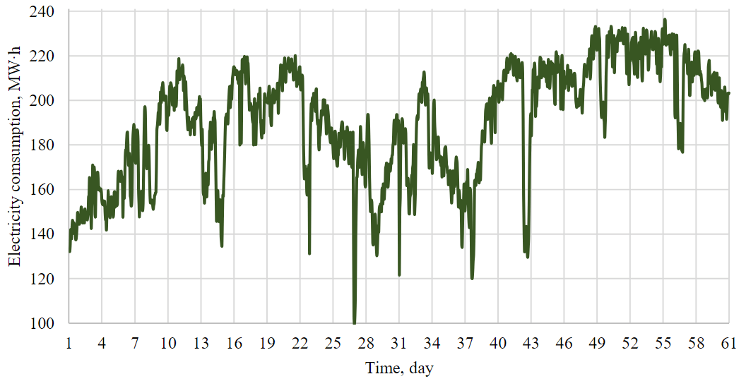
Fig.1. Fragment of the enterprise's electricity consumption graph
Dataset formation for machine learning application
Time series forecasting using machine learning models, one of the key factors affecting the result is the selection of features [14, 16, 34]. Typically, in addition to other features, electricity consumption forecasting uses previous values to predict subsequent ones:
where yi* is the forecasted electricity consumption at i time; f is the forecasting model; g is a function that defines the rule for selecting retrospective actual electricity consumption values; h is the forecasting horizon; w – is the width of the retrospective data window; X are other features (e.g., hour or day of the week, meteorological factors, production factors, etc.).
When using neural network models, especially recurrent ones, it is possible to process all values of the time series yi-h, yi-h-1,...,yi-h-w [5, 6, 21]. However, for industrial enterprises, it is sufficient to use retrospective time series values that are offset from the forecasted hour by a multiple of 6, 12, or 24 h, which is related to production technological cycles. This allows for significantly simplifying the model and reducing the risk of overfitting due to an excessive number of features [6, 16, 35].
During preliminary correlation analysis, it was determined that for forecasting, it is sufficient to use hours with a step of 12 and a retrospective depth of three days. For example, to forecast the daily load profile component for 28.10.2023 from 19:00 to 20:00, the following data will be used: electricity consumption from 27.10.2023 from 19:00 to 20:00 and 07:00 to 08:00, from 26.10.2023 from 19:00 to 20:00, and from 25.10.2023 from 19:00 to 20:00. Thus, the expression takes the form:
where X contains the following features: hour number i (from 0 to 23); day of the month for the forecast (from 1 to 31); day of the week for the forecast (1-7); month for the forecast (1-12); expert-manual load forecast yei (results were obtained with and without its consideration); wind speed at hour i; air temperature at hour i; atmospheric pressure at hour i; relative humidity at hour i; scheduled repairs, vector rij, j = 1, … m.
As a result, the full feature vector contains 37 values (5 retrospective electricity consumption values; 4 calendar features; expert-manual load forecast; 4 meteorological factors; 23 repair-related features). During the study, various combinations of features were tested to determine their impact on forecast accuracy. Data preprocessing, model building, and testing were performed in Python 3 using the open-source Pandas and Scikit-Learn libraries.
Used machine learning methods
Short-term electricity consumption forecasting for enterprises is effectively addressed using artificial neural networks and decision tree ensembles. Previous research by the authors of this article demonstrated that ensemble models of gradient and adaptive boosting, as well as random forests, achieve comparable accuracy to neural network models while offering faster training times and simpler hyperparameter tuning [6, 16, 33]. Studies [27, 29] successfully applied decision tree ensembles for forecasting electricity consumption.
Therefore, in this work, ensemble methods including random forest (Random Forest) and adaptive boosting (AdaBoost), extreme gradient boosting (XGBoost) [36] for building ensembles of regression decision trees. A single tree can be represented as
where t is a hierarchical system of rules, each comparing the value of a specific feature to a threshold.
Random forest builds a regression model as an ensemble of k decision trees, each trained independently on a randomly selected subset of instances from the training dataset:
In contrast, adaptive boosting and extreme gradient boosting build ensembles iteratively. Each subsequent model in the ensemble depends on the results of previous ones. Ultimately, the model is formed as
where wj is the weight of the j-й model (in this case, a decision tree).
After adding each new model to the ensemble, adaptive boosting adjusts the weights of the training dataset instances, increasing them proportionally to the deviation of the model's output from the true value. In gradient boosting, the gradient of the error of the current ensemble serves as the optimization criterion for building each new model in the ensemble. Various implementations of gradient boosting exist, including extreme boosting [36].
Analysis of the applicability of eXplainable Artificial Intelligence
The use of systems that provide experts with decisions without explanations based on non-interpretable algorithms is limited because they lack user trust and may contain hidden risks of unforeseen critical errors. To address this issue, the field of research focusing on improving user interaction with intelligent systems through eXplainable Artificial Intelligence (XAI) methods is developing. XAI aims to create intelligent systems capable of interpreting their results and explaining them to the user [37, 38]. The XAI concept involves adhering to principles of explainability (the intelligent system must explain its results), significance (the explanation should be tailored for the user), accuracy (the explanation should truthfully describe how the model obtained the result), and limits of knowledge (the intelligent system must understand its applicability boundaries and not attempt to solve tasks beyond its capabilities).
The directions of XAI application can be divided into creating self-interpretable models and methods of a posteriori explanation of obtained results. For example, a decision tree with a small depth is an interpretable model because it represents a system of rules. For complex tasks, current methods use non-interpretable models, employing the second approach – applying a posteriori explanation method. Among such explanation methods, there is the Local Interpretable Model-Agnostic Explanations (LIME) method [39]. LIME involves building a local surrogate model that explains the workings of the explainable model in a narrow neighborhood of the considered input instance. The local surrogate model is a simple, interpretable model, such as a decision tree or linear regression, trained to predict the output of the explainable model in this neighborhood. A limitation of the method is the need to select, tune, and train the surrogate model, as well as the implicit violation of the accuracy principle, as the hypothesis that the surrogate model's explanation corresponds to the decision-making mechanism of the explainable model is an unverifiable assumption in each specific case.
For convolutional neural networks, methods based on class activation mapping (CAM), such as Grad-CAM, are used [40]. A limitation of this method is its applicability only to convolutional neural networks, as it relies on processing feature maps formed by each convolutional layer and calculating gradients derived from the model's output results with respect to the feature maps.
If the user of an intelligent decision support system is an expert in the solved task, displaying features that influenced the decision formation along with their significance (weights) increases trust in the system and the likelihood of effective collaborative work with it. Therefore, in such areas as diagnostics, planning, or forecasting, where the model is used by an expert, the application of the additive SHAP (SHapley Additive exPlanations) method based on the Shapley vector is particularly relevant [41]. The additive SHAP explanation is based on the Shapley values algorithm from game theory. It determines the contribution of each player to the overall winnings. If players are replaced by features and winnings by the machine learning model's results, an algorithm for determining the impact of each feature on the model's result is obtained. When using the SHAP algorithm, the significance of the j-th feature for the model f when analyzing input data Zi is calculated as:
where m is the number of features; S is a subset of features; P is the set of all possible feature combinations; i is the input data instance; j is the feature index. If a feature is not used, its value is replaced with the average value. As a result, the feature's importance j is assessed by analyzing its impact on the model's results with and without it for various sets of other features.
The application of LIME and SHAP methods in power industry is still in its initial stages. In [42], both methods are applied to solar power plant generation forecasting. SHAP is used for electricity consumption forecasting in [43], but the object is a large energy system, not a specific enterprise.
In this work, for the first time, the principles of an intelligent system for short-term forecasting of electrical power consumption of a mining enterprise, considering meteorological factors and scheduled repairs, which provides the user with a forecast justification using the additive SHAP explanation were proposed and validated. The analysis of the obtained explanations and the description of the specialist's interaction with the intelligent system in load planning were presented.
Discussion
Results of electricity consumption forecast
The performance metrics of AdaBoost, XGBoost, and Random Forest methods for forecasting of electrical consumption were compared to the load forecast error manually created by an expert: mean absolute error (MAE) – 16.53 MW·h; mean absolute percentage error (MAPE) – 9.85 %; root mean square error (RMSE) – 21.18 MW·h. The dataset for model construction was divided into training and test sets with a 90:10 ratio.
Experiments to build machine learning models for forecasting the electrical consumption of a mining enterprise, considering different features were conducted.
In the first experiment, the following features were chosen:
- hour number i (from 0 to 23);
- day of the month for the forecast (from 1 to 31);
- day of the week for the forecast (1-7);
- month for the forecast (1-12);
- retrospective electricity consumption (consumption_1, consumption_2, consumption_3, consumption_4, consumption_5 – yi-24, yi-36,yi-48, yi-60, yi-72).
Table 2 presents the forecasting results for electricity consumption using these features. Used notations are max_depth – maximum depth of decision trees in the ensemble; n_estimators – number of trees in the ensemble. The AdaBoost method achieved the best MAPE for the test set – 9.68 %. Compared to the MAPE of forecast manually created by an expert (9.85 %), the accuracy improved by 0.17 %. It can be concluded that without additional consideration of technological process parameters and metrological factors, the application of machine learning models does not enhance the accuracy of electricity consumption forecasting. However, it reduces the time required to obtain the result. An expert takes 2-4 h to compile a consumption graph, whereas training takes up to 5 min.
Table 2
Forecasting of electricity consumption of the enterprise with consideration of retrospective consumption
|
Method |
MAE, MW·h |
MAPE, % |
RMSE, MW·h |
max_depth |
n_estimators |
|||
|
Training |
Test |
Training |
Test |
Training |
Test |
|||
|
AdaBoost |
10.28 |
15.80 |
8.88 |
9.68 |
12.51 |
20.96 |
7 |
200 |
|
XGBoost |
9.09 |
18.45 |
8.34 |
11.58 |
12.84 |
23.79 |
3 |
150 |
|
Random Forest |
10.60 |
17.07 |
9.96 |
10.89 |
15.30 |
23.56 |
7 |
7 |
In the second experiment, the feature vector rij, j = 1, … m of scheduled repairs was added to the features selected in first experiment (Table 3).
Table 3
Forecasting of electricity consumption of the enterprise with consideration of retrospective consumption and scheduled repairs
|
Method |
MAE, MW·h |
MAPE, % |
RMSE, MW·h |
max_depth |
n_estimators |
|||
|
Training |
Test |
Training |
Test |
Training |
Test |
|||
|
AdaBoost |
10.27 |
17.15 |
8.93 |
10.40 |
12.51 |
22.23 |
7 |
200 |
|
XGBoost |
10.71 |
17.24 |
9.76 |
10.72 |
15.06 |
22.63 |
2 |
150 |
|
Random Forest |
11.28 |
18.26 |
10.61 |
11.39 |
16.32 |
24.34 |
6 |
150 |
Similarly to the first experiment, the AdaBoost method achieved the best MAPE for the test set – 10.40 %. Incorporating the scheduled repairs factor degraded the forecast accuracy by 0.55 %, contrary to expectations of improved accuracy with additional consideration of production process factors. Further experiments with various repair grouping variants (feature aggregations) did not yield accuracy improvements. This is due to discrepancies between scheduled and actual repairs. For instance, if a repair was scheduled for 2 h from 10:00 to 12:00, it might have occurred at a different time (e.g., 14:00 to 16:00) or lasted longer (e.g., 10:00 to 17:00).
In the future, it may be beneficial to consider only repairs scheduled with high accuracy, such as those lasting several days. This would reduce the stochastic impact of short repairs on the electricity consumption graph.
In the third experiment, meteorological parameters for the i-th hour (wind speed, air temperature, atmospheric pressure, and humidity) were added to the features selected for the first experiment (Table 4).
Table 4
Forecasting of electricity consumption of the enterprise with consideration of retrospective consumption and meteorological factors
|
Method |
MAE, MW·h |
MAPE, % |
RMSE, MW·h |
max_depth |
n_estimators |
|||
|
Training |
Test |
Training |
Test |
Training |
Test |
|||
|
AdaBoost |
9.44 |
13.14 |
8.17 |
8.17 |
11.39 |
17.66 |
7 |
200 |
|
XGBoost |
8.12 |
12.89 |
7.57 |
7.85 |
11.49 |
17.18 |
3 |
150 |
|
Random Forest |
8.79 |
13.59 |
8.37 |
8.73 |
12.70 |
18.93 |
8 |
150 |
In the fourth experiment, both scheduled repairs and meteorological factors were considered (Table 5). The AdaBoost method achieved the best MAPE for the test set – 8.38 %. Although this represents a 1.48 % improvement over the forecast manually created by an expert, it is primarily due to the inclusion of meteorological factors. The discrepancy between actual and scheduled repairs prevents the use of repair data for model construction.
Table 5
Forecasting of electricity consumption of the enterprise with consideration of retrospective consumption, scheduled repairs, and meteorological factors
|
Method |
MAE, MW·h |
MAPE, % |
RMSE, MW·h |
max_depth |
n_estimators |
|||
|
Training |
Test |
Training |
Test |
Training |
Test |
|||
|
AdaBoost |
8.31 |
13.57 |
8.03 |
8.38 |
11.22 |
18.10 |
7 |
200 |
|
XGBoost |
7.93 |
14.73 |
7.38 |
9.13 |
11.29 |
19.26 |
3 |
150 |
|
Random Forest |
8.72 |
14.38 |
8.32 |
9.04 |
12.56 |
19.57 |
8 |
150 |
In the fifth experiment, retrospective consumption data, meteorological factors, and the forecast manually created by an expert were used (Table 6). Additionally, computational experiments with long short-term memory neural networks, specifically, Gated Recurrent Units (GRU), were conducted for model applicability assessment, following the architecture and hyperparameter selection approach described in [5]. The XGBoost method yielded the best MAPE for the test set – 7.41 %. This represents a 2.44 % improvement over the manually conducted expert forecast (9.85 %). In an intelligent system, integrating the expert forecast can be achieved through two methods: applying expert adjustments to the model-generated load curve; refining the expert load curve using the model.
The first method is preferable as it saves the time the expert spends on creating the planned electricity consumption load curve.
Table 6
Forecasting of electricity consumption of the enterprise with consideration of retrospective consumption, meteorological factors, and the forecast manually created by an expert
|
Method |
MAE, MW·h |
MAPE, % |
RMSE, MW·h |
max_depth |
n_estimators |
|||
|
Training |
Test |
Training |
Test |
Training |
Test |
|||
|
AdaBoost |
8.06 |
13.63 |
6.79 |
8.35 |
9.67 |
17.91 |
7 |
200 |
|
XGBoost |
8.29 |
11.94 |
7.29 |
7.41 |
11.85 |
16.53 |
2 |
150 |
|
Random Forest |
9.50 |
13.14 |
8.26 |
8.30 |
13.71 |
17.84 |
5 |
150 |
|
GRU |
8.11 |
13.16 |
7.15 |
8.31 |
11.52 |
17.80 |
– |
– |
Figure 2 compares actual and forecasted electricity consumption. Analysis of the load curves indicates that incorporating and the forecast manually created by an expert allows the machine learning model to more accurately forecast sudden aperiodic consumption changes, highlighted by red ovals. Future research could focus on identifying and formalizing production factors related to these technological process changes, and integrating these factors as additional features into the machine learning model.
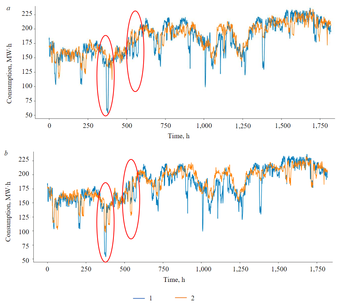
Fig.2. Comparison of actual (1) and forecasted (2) consumption considering: retrospective consumption and meteorological parameters (a); retrospective consumption, meteorological parameters, and the forecast manually created by an expert (b)
Table 7 summarizes the experimental results. Absolute and relative forecast improvements were calculated relative to the MAPE of the forecast manually created by an expert (9.85 %). Considering additional factors enhances accuracy. With retrospective consumption and meteorological data, forecast accuracy improves by 20.34 %. Including the forecast manually created by an expert, it further increases accuracy by 24.75 %.
Table 7
Forecasting of electricity consumption of the enterprise with consideration of different features
|
Experiment |
Feature under consideration |
Model |
MAPE, % |
Absolute forecast improvement |
Relative forecast improvement |
|
1 |
Retrospective consumption |
AdaBoost |
9.68 |
0.17 |
1.70 |
|
2 |
Retrospective consumption, scheduled repairs |
AdaBoost |
10.40 |
–0.55 |
–5.54 |
|
3 |
Retrospective consumption, meteorological factors |
XGBoost |
7.85 |
2.00 |
20.34 |
|
4 |
Retrospective consumption, meteorological factors, and scheduled repairs |
AdaBoost |
8.38 |
1.48 |
14.97 |
|
5 |
Retrospective consumption, meteorological factors, and forecast manually created by an expert |
XGBoost |
7.41 |
2.44 |
24.75 |
Explanation of results
SHAP enables the formal mapping of features that influenced the forecast of electricity consumption for each hour, along with their significance (weights), which can be interpreted by an expert.
Figure 3 illustrates the features affecting the electricity consumption forecast for one hour during the winter period in the third experiment, which considered retrospective consumption and meteorological factors. Features are arranged in descending order of their impact on the deviation of the forecasted consumption f(x) from the average value E[f(x)]. Thus, for the data in Fig.3, it can be concluded that the deviation of f(x), which was 177.665 MW·h, from the average value of 136.496 MW·h, is justified by high consumption 24, 36, and 48 h before the forecasted hour and low air temperature.
Figure 4 shows the features affecting the electricity consumption forecast for another hour during the winter period in the same experiment. The deviation of f(x), which was 213.972 MW·h, from the average value of 136.496 MW·h, is justified by abnormally low air temperature and high consumption 24, 36, and 72 h before the forecasted hour.
Figure 5 depicts the features affecting the electricity consumption forecast during the winter period in the same experiment with a different distribution of significance for meteorological features. The deviation of f(x), which was 190.858 MW·h, from the average value of 136.496 MW·h, is justified by consumption 24, 36, and 72 h before the forecasted hour, air temperature, as well as wind speed and pressure values. The analysis of features obtained using the Shapley method confirms the necessity of considering meteorological factors when building a model for forecasting electricity consumption.
Figure 6 presents the results for the fifth experiment, where the expert-formulated consumption plan was considered for the same hour analyzed in Fig.3. The expert-formulated plan itself contributed the most to the value of f (x), which was 180.863 MWh. However, the meteorological factors also play a crucial role even when considering the expert-formulated consumption plan, as shown in Fig.7 for the same hour analyzed in Fig.4.
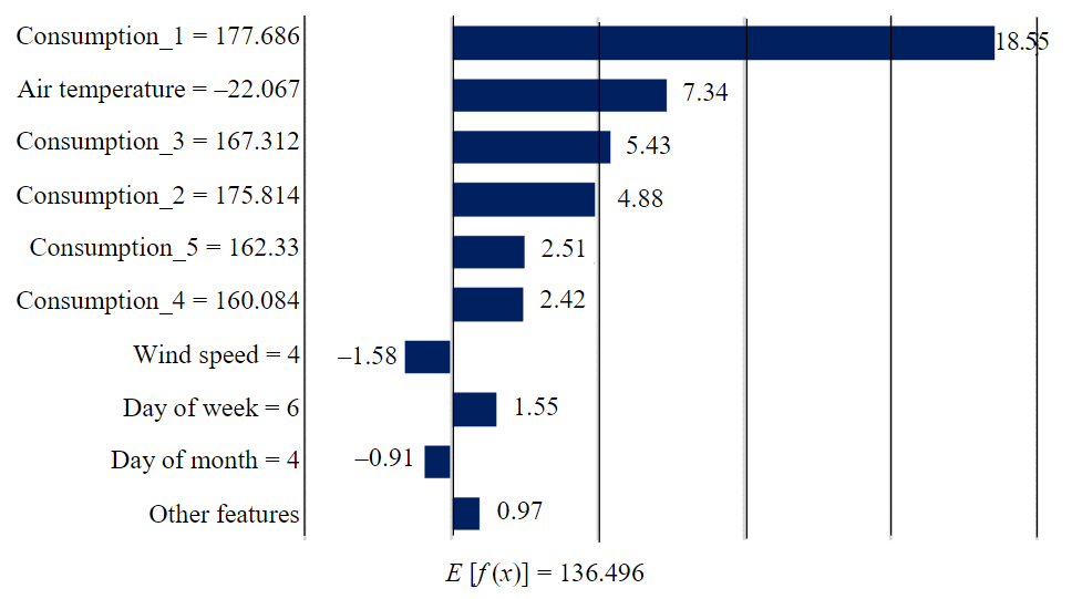
Fig.3. Visualization of features impacting the electricity consumption forecastf (x) = 177.665 MW·h
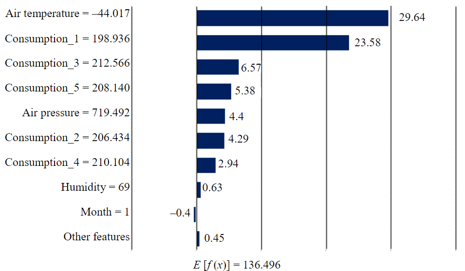
Fig.4. Visualization of features impacting the electricity consumption forecastf (x) = 213.972 MW·h
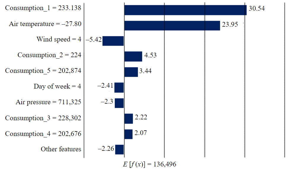
Fig.5. Visualization of features impacting the electricity consumption forecastf (x) = 190.858 MW·h
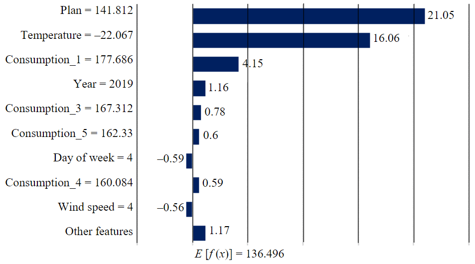
Fig.6. Visualization of features impacting the electricity consumption forecastf (x) = 180.863 MW·h
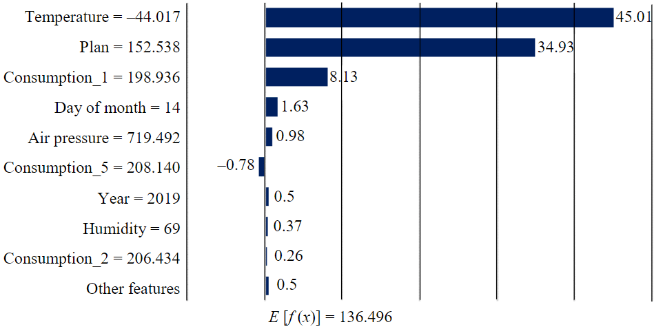
Fig.7. Visualization of features impacting the electricity consumption forecastf (x) = 227.987 MW·h
The experiments conducted demonstrate that the SHapley Additive exPlanations for each output value of the machine learning model visually and comprehensibly illustrates the feature impacts, enhancing the model's interpretability for experts. It should be noted that this result does not fully meet the requirements for explainable artificial intelligence outlined above. Nonetheless, the SHapley Additive exPlanations is considered one of the most promising methods in explainable artificial intelligence, and its further development in forecasting tasks will likely increase the trust of electricity consumption experts in machine learning-based systems.
Conclusion
An approach to creating an intelligent system for short-term forecasting of electricity consumption of a mining enterprise, considering meteorological factors and scheduled repairs was proposed. Incorporating meteorological factors in addition to consumption history enhances forecast accuracy by 20.34 %.
However, due to discrepancies between actual and planned repairs, forecast accuracy decreases by 0.55 % relative to the forecast manually created by an expert when considering scheduled repairs. Future research will focus on accounting only for repairs lasting more than 12 h to minimize the impact of inaccurate repair forecasts on model training results.
Applying an expert-formulated plan along with retrospective consumption and meteorological factors increases forecast accuracy to 24.75 %. In developing an information system, this expert plan can be incorporated through expert correction functions and analysis of historical discrepancies between expert corrections and model results. Future research also aims to more precisely formalize expert experience.
The proposed approach to creating an information system includes a model that provides users with a forecast justification using SHapley Additive exPlanations. Explanation results enable experts to analyze the impact of factors on forecasting results, simplifying the introduction of expert corrections and accelerating system implementation. The practical significance of the study lies in enhancing the accuracy of short-term electricity consumption forecasting for industrial enterprises by considering equipment repairs and shutdowns and creating conditions for industry-wide adoption of machine learning-based information systems using explainable artificial intelligence algorithms, thereby increasing user trust.
The proposed system is planned to be tested using machine learning methods and explainable machine learning models on data from other industrial enterprises with larger volumes of available indicator data and deeper historical depth; to specify and formalize production factors for their inclusion as model features; modify the SHapley Additive exPlanations to improve the interpretability of its results for the considered task; and analyze the impact of electricity consumption forecast accuracy on the enterprise's electricity consumption costs.
References
- Park S., Ruy S., Choi Y. et al. Data-Driven Baseline Estimation of Residential Buildings for Demand Response. Energies. 2015. Vol. 8. Iss. 9, p. 10239-10259. DOI: 10.3390/en80910239
- Almuhaini S.H., Sultana N. Forecasting Long-Term Electricity Consumption in Saudi Arabia Based on Statistical and Machine Learning Algorithms to Enhance Electric Power Supply Management. Energies. 2023. Vol. 16. Iss. 4. N 2035. DOI: 10.3390/en16042035
- Faria P., Vale Z. Demand Response in Smart Grids. Energies. 2023. Vol. 16. Iss. 2. N 863. DOI: 10.3390/en16020863
- Kanapelko R.A. Russian and foreign practice of interaction between corporate and government structures of the wholesale electricity and capacity market. Journal of Economy and Business. 2019. N 2, p. 47-51 (in Russian). DOI: 10.24411/2411-0450-2019-10364
- Matrenin P.V., Manusov V.Z., Khalyasmaa A.I. et al. Improving Accuracy and Generalization Performance of Small-Size Recurrent Neural Networks Applied to Short-Term Load Forecasting. Mathematics. 2020. Vol. 8. Iss. 12. N 2169. DOI: 10.3390/math8122169
- Antonenkov D.V., Matrenin P.V. Ensemble and Neural Network Machine Learning Models for Short-Term Load Forecasting of Open Cast Mining Companies. Electrotechnical Systems and Complexes. 2021. N 3 (52), p. 57-65 (in Russian). DOI: 10.18503/2311-8318-2021-3(52)-57-65
- Nepsha F.S., Krasilnikov M.I., Perevalov K.V. Application of a digital platform to build intelligent energy management systems for mining enterprises. Avtomatizatsiya i IT v energetike. 2021. N 5 (142), p. 26-34. (in Russian)
- Jianjun Fan, Xinzhong Liu, Zhimin Li et al. Power load forecasting research based on neural network and Holt-winters method. IOP Conference Series: Earth and Environmental Science. 2021. Vol. 692. N 022120. DOI: 10.1088/1755-1315/692/2/022120
- Potapov V., Khamitov R., Makarov V. et al. Short-Term Forecast of Electricity Load for LLC “Omsk Energy Retail Company” Using Neural Network. 2018 Dynamics of Systems, Mechanisms and Machines (Dynamics), 13-15 November 2018, Omsk, Russia. IEEE, 2018. DOI: 10.1109/Dynamics.2018.8601430
- Chodakowska E., Nazarko J., Nazarko Ł. ARIMA Models in Electrical Load Forecasting and Their Robustness to Noise. Energies. 2021. Vol. 14. Iss. 23. N 7952. DOI: 10.3390/en14237952
- Sharma S., Majumdar A., Elvira V., Chouzenoux É. Blind Kalman Filtering for Short-Term Load Forecasting. IEEE Transactions on Power Systems. 2020. Vol. 35. Iss. 6, p. 4916-4919. DOI: 10.1109/TPWRS.2020.3018623
- Madhukumar M., Sebastian A., Xiaodong Liang et al. Regression Model-Based Short-Term Load Forecasting for University Campus Load. IEEE Access. 2022. Vol. 10, p. 8891-8905. DOI: 10.1109/ACCESS.2022.3144206
- Serebryakov N.A. Application of Deep Neural Network Ensemble in a Problem of Short-Term Load Forecasting Guaranteed Electricity Supplier. Electrotechnical Systems and Complexes. 2021. N 2 (51), p. 52-60 (in Russian). DOI: 10.18503/2311-8318-2021-2(51)-52-60
- Caro E., Juan J., Nouhitehrani S. Optimal Selection of Weather Stations for Electric Load Forecasting. IEEE Access. 2023. Vol. 11, p. 42981-42990. DOI: 10.1109/ACCESS.2023.3270933
- Sergeev N., Matrenin P. Improving Accuracy of Machine Learning Based Short-Term Load Forecasting Models with Correlation Analysis and Feature Engineering. 2023 IEEE 24th International Conference of Young Professionals in Electron Devices and Materials (EDM), 29 June – 3 July 2023, Novosibirsk, Russia. IEEE, 2023, p. 1000-1004. DOI: 10.1109/EDM58354.2023.10225058
- Habbak H., Mahmoud M., Metwally K. et al. Load Forecasting Techniques and Their Applications in Smart Grids. Energies. 2023. Vol. 16. Iss. 3. N 1480. DOI: 10.3390/en16031480
- Ryu S., Noh J., Kim H. Deep Neural Network Based Demand Side Short Term Load Forecasting. Energies. 2017. Vol. 10. Iss. 1. N 3. DOI: 10.3390/en10010003
- Szczepaniuk H., Szczepaniuk E.K. Applications of Artificial Intelligence Algorithms in the Energy Sector. Energies. 2023. Vol. 16. Iss. 1. N 347. DOI: 10.3390/en16010347
- Lizhen Wu, Chun Kong, Xiaohong Hao, Wei Chen. A Short-Term Load Forecasting Method Based on GRU-CNN Hybrid Neural Network Model. Mathematical Problems in Engineering. 2020. Vol. 2020. Iss. 1. N 1428104. DOI: 10.1155/2020/1428104
- Zhuofu Deng, Binbin Wang, Yanlu Xu et al. Multi-Scale Convolutional Neural Network With Time-Cognition for Multi-Step Short-Term Load Forecasting. IEEE Access. 2019. Vol. 7, p. 88058-88071. DOI: 10.1109/ACCESS.2019.2926137
- Weicong Kong, Zhao Yang Dong, Youwei Jia et al. Short-Term Residential Load Forecasting Based on LSTM Recurrent Neural Network. IEEE Transactions on Smart Grid. 2019. Vol. 10. Iss. 1, p. 841-851. DOI: 10.1109/TSG.2017.2753802
- Potapov V.I., Gritsay A.S., Tyunkov D.A., Sinitsin G.E. Using neural network for building short-term forecast of electricity load of LLC “Omsk Energy Retail Company”. Bulletin of the Tomsk Polytechnic University. Geo Аssets Engineering. 2016. Vol. 327. N 8, p. 44-51 (in Russian).
- Cai M., Pipattanasomporn M., Rahman S. Day-ahead building-level load forecasts using deep learning vs. traditional time-series techniques. Applied Energy. 2019. Vol. 236, p. 1078-1088. DOI: 10.1016/j.apenergy.2018.12.042
- Ye Hong, Yingjie Zhou, Qibin Li et al. A Deep Learning Method for Short-Term Residential Load Forecasting in Smart Grid. IEEE Access. 2020. Vol. 8, p. 55785-55797. DOI: 10.1109/ACCESS.2020.2981817
- Zhuofu Deng, Binbin Wang, Yanlu Xu et al. Multi-Scale Convolutional Neural Network With Time-Cognition for Multi-Step Short-Term Load Forecasting. IEEE Access. 2019. Vol. 7, p. 88058-88071. DOI: 10.1109/ACCESS.2019.2926137
- Ahmad N., Ghadi Y., Adnan M., Ali M. Load Forecasting Techniques for Power System: Research Challenges and Survey. IEEE Access. 2022. Vol. 10, p. 71054-71090. DOI: 10.1109/ACCESS.2022.3187839
- Klyuev R.V., Morgoeva A.D., Gavrina O.A. et al. Forecasting planned electricity consumption for the united power system using machine learning. Journal of Mining Institute. 2023. Vol. 261, p. 392-402.
- Rusina A.G., Filippova T.A., Kalinin A.E., Terlyga N.S. Short-Term Electricity Consumption Forecast in Siberia IPS Using Climate Aspects. 2018 19th International Conference of Young Specialists on Micro/Nanotechnologies and Electron Devices (EDM), 29 June – 3 July 2018, Erlagol, Russia. IEEE, 2018, p. 6403-6407. DOI: 10.1109/EDM.2018.8435002
- Morgoev I.D., Dzgoev A.E., Klyuev R.V., Morgoeva A.D. Forecasting of electricity consumption by enterprises of the public sector complex in conditions of incomplete information. Izvestiya Kabardino-Balkarskogo nauchnogo tsentra RAS. 2022. N 3 (107), p. 9-20 (in Russian). DOI: 10.35330/1991-6639-2022-3-107-9-20
- Antonenkov D.V., Solovev D.B. Mathematic simulation of mining company’s power demand forecast (by example of “Neryungri” coal strip mine). IOP Conference Series: Earth and Environmental Science. 2017. Vol. 87. Iss. 3. N 032003. DOI: 10.1088/1755-1315/87/3/032003
- Morgoeva A.D., Morgoev I.D., Klyuev R.V., Gavrina O.A. Forecasting of electric energy consumption by an industrial enterprise using machine learning methods. Bulletin of the Tomsk Polytechnic University. Geo Аssets Engineering. 2022. Vol. 333. N 7, p. 115-125 (in Russian). DOI: 10.18799/24131830/2022/7/3527
- Vyalkova S.A., Morgoeva A.D., Gavrina O.A. Development of a hybrid model for predicting the consumption of electrical energy for a mining and metallurgical enterprise. Sustainable Development of Mountain Territories. 2022. Vol. 14. N 3 (53), p. 486-493 (in Russian). DOI: 10.21177/1998-4502-2022-14-3-486-493
- Khalyasmaa A., Matrenin P. Initial Data Corruption Impact on Machine Learning Models’ Performance in Energy Consumption Forecast. 2021 Ural-Siberian Smart Energy Conference (USSEC), 13-15 November 2021, Novosibirsk, Russian Federation. IEEE, 2021, p. 5. DOI: 10.1109/USSEC53120.2021.9655724
- Bouktif S., Fiaz A., Ouni A., Serhani M.A. Optimal Deep Learning LSTM Model for Electric Load Forecasting using Feature Selection and Genetic Algorithm: Comparison with Machine Learning Approaches. Energies. 2018. Vol. 11. Iss. 7. N 1636. DOI: 10.3390/en11071636
- Manusov V.Z. Neural networks: forecasting of electrical loads and power losses in electric grids. From romanticism to pragmatism. Novosibirsk: NSTU Publisher, 2018, p. 303 (in Russian).
- Tianqi Chen, Guestrin C. XGBoost: A Scalable Tree Boosting System. KDD’16: Proceedings of the 22nd ACM SIGKDD International Conference on Knowledge Discovery and Data Mining, 13-17 August 2016, San Francisco, CA, USA. New York: Association for Computing Machinery, 2016, p. 785-794. DOI: 10.1145/2939672.2939785
- Ahmed I., Jeon G., Piccialli F. From Artificial Intelligence to Explainable Artificial Intelligence in Industry 4.0: A Survey on What, How, and Where. IEEE Transactions on Industrial Informatics. 2022. Vol. 18. Iss. 8, p. 5031-5042. DOI: 10.1109/TII.2022.3146552
- Adadi A., Berrada M. Peeking Inside the Black-Box: A Survey on Explainable Artificial Intelligence (XAI). IEEE Access. 2018. Vol. 6, p. 52138-52160. DOI: 10.1109/ACCESS.2018.2870052
- Ribeiro M.T., Singh S., Guestrin C. “Why Should I Trust You?”: Explaining the Predictions of Any Classifier. The 2016 Conference of the North American Chapter of the Association for Computational Linguistics: Human Language Technologies. Proceedings of the Demonstrations Session, 12-17 June 2016, San Diego, CA, USA. Stroudsburg: Association for Computational Linguistics, 2016, p. 97-101. DOI: 10.48550/arXiv.1602.04938
- Selvaraju R.R., Cogswell M., Das A. et al. Grad-CAM: Visual Explanations from Deep Networks via Gradient-Based Localization. International Journal of Computer Vision. 2020. Vol. 128. Iss. 2, p. 336-359. DOI: 10.1007/s11263-019-01228-7
- Lundberg S.M., Su-In Lee. A unified approach to interpreting model predictions. NIPS’17: Proceedings of the 31st International Conference on Neural Information Processing Systems, 4-9 December 2017, Long Beach, CA, USA. Red Hook: Curran Associates Inc., 2017, p. 4768-4777. DOI: 10.48550/arXiv.1705.07874
- Kuzlu M., Cali U., Sharma V., Güler Ö. Gaining Insight Into Solar Photovoltaic Power Generation Forecasting Utilizing Explainable Artificial Intelligence Tools. IEEE Access. 2020. Vol. 8, p. 187814-187823. DOI: 10.1109/ACCESS.2020.3031477
- Hengbo Liu, Ziqing Ma, Linxiao Yang et al. SADI: A Self-Adaptive Decomposed Interpretable Framework for Electric Load Forecasting Under Extreme Events. ICASSP 2023 – 2023 IEEE International Conference on Acoustics, Speech and Signal Processing, 4-10 June 2023, Rhodes Island, Greece. IEEE, 2023, p. 5. DOI: 10.1109/ICASSP49357.2023.10096002
