
Investigation of the accuracy of constructing digital elevation models of technogenic massifs based on satellite coordinate determinations
- 1 — Ph.D., Dr.Sci. Professor Emperor Alexander I St. Petersburg State Transport University ▪ Orcid
- 2 — Ph.D., Dr.Sci. Head of Department Empress Catherine II Saint Petersburg Mining University ▪ Orcid
- 3 — Ph.D. Principal Discipline Engineer AO “Gazprom Diagnostika” ▪ Orcid
- 4 — Ph.D. Leading Engineer Empress Catherine II Saint Petersburg Mining University ▪ Orcid
Abstract
At all stages of the life cycle of buildings and structures, geodetic support is provided by electronic measuring instruments – a laser scanning system, unmanned aerial vehicles, and satellite equipment. In this context, a set of geospatial data is obtained that can be presented as a digital model. The relevance of this work is practical recommendations for constructing a local quasigeoid model and a digital elevation model (DEM) of a certain accuracy. A local quasigeoid model and a DEM were selected as the study objects. It is noted that a DEM is often produced for vast areas, and, therefore, it is necessary to build a local quasigeoid model for such models. The task of assessing the accuracy of constructing such models is considered; its solution will allow obtaining a better approximation to real data on preassigned sets of field materials. A general algorithm for creating both DEM and local quasigeoid models in the Golden Software Surfer is presented. The constructions were accomplished using spatial interpolation methods. When building a local quasigeoid model for an area project, the following methods were used: triangulation with linear interpolation (the least value of the root mean square error (RMSE) of interpolation was 0.003 m) and kriging (0.003 m). The least RMSE value for determining the heights by control points for an area project was obtained using the natural neighbour (0.004 m) and kriging (0.004 m) methods. To construct a local quasigeoid model for a linear project, the following methods were applied: kriging (0.006 m) and triangulation with linear interpolation (0.006 m). Construction of the digital elevation model resulted in the least aggregate value of the estimated parameters: on a flat plot of the earth’s surface – the natural neighbour method, for a mountainous plot with anthropogenic topography – the quadric kriging method, for a mountainous plot – quadric kriging.
None
Introduction
Geodetic support, which includes engineering and geodetic survey, siting work, and pre-construction survey, is an important aspect of ensuring the design, construction and operation of buildings and structures, including projects in the mineral resources sector. During operation, monitoring of the facility deformations can be carried out [1]. At all life cycle stages of mineral resource sector projects it is possible to use the advanced technologies: information [2, 3], numerical [4-6] and simulation modelling [7] as well as neural networks [8, 9]. In this case, it is possible to monitor the main characteristics of the investigated project in a safe manner and in great detail, which leads to quality improvement of the handed-over field materials and an expansion of the information set regarding the research object. In respect of geodetic support of the work, the use of advanced technologies allows combining geospatial data into a single set of reliable information used for taking engineering decisions and creating integrated models for safe operation of engineering constructions [10-12]. Non-contact methods of terrain surveying, such as laser scanning [13] and photogrammetric me-thods [14] including unmanned aerial vehicles [15-17] are actively applied. It should be noted that lately the observation methods with a satellite navigation system (GNSS) were applied to determine the altitude position of structural elements [18] for the efficient use of which it is necessary to have a quasigeoid height model or a height anomaly model for the construction site. It should be emphasized that in the process of designing and constructing the projects as well as in various urban development works, including land development, generation of a digital elevation model (DEM) based on the obtained data is an important stage for obtaining spatial information about the work site. Assessment of the accuracy and automation of DEM creation is a relevant task, since the quality and speed of construction allow increasing the productivity of all the related processes. Thus, the task of studying the accuracy of producing a local quasigeoid model and DEM arises in the absence of general recommendations for their construction [19, 20] and accuracy assessment [21, 22]. For example, articles [23-25] contain recommendations on the use of spatial interpolation methods [26, 27] for producing mathematical elevation models.
It should be noted that the construction of DEM is possible both with and without using a local quasigeoid model. However, this can lead to distortion of the information on topography [19, 25]. To provide the results of geodetic support, the normal height system is used [18, 28, 29]. In case of obtaining geodetic heights, the question of switching to it arises. Then, a local quasigeoid model is needed [30-32] for the creation of which it is important to have combined points [33, 34] (with known geodetic heights from the GNSS definitions and normal or orthometric heights from geometric levelling). Modelling of the surface of height anomalies [34] was caused primarily by land planning in Poland [28], Slovenia [31], coastal cities of the Red Sea [20], and Ethiopia [34].
The authors of [21, 35] noted that the production of such models in hard-to-reach mountainous areas is an important stage in accurate determination of heights using the GNSS equipment. Article [28] indicates that an accuracy of 5 mm was attained when creating a local model for the territory of Krakow. The production of such models is important for development of the regions [33]. Often, the problem of modelling the surface of height anomalies for an area project is solved. However, there are no studies aimed at creating a local quasigeoid model for an extensive linear project. No recommendations were drawn up concerning the required number of points or the method for assigning a sufficient number of points to create a model in which the accuracy of determining the heights would correspond to the accuracy indicated in work specifications at each stage of construction.
When determining the corrections to geodetic heights for further construction of DEM, it is necessary to choose the spatial interpolation method that will be used to construct a mathematical model of height anomalies [36]. DEM construction from data obtained by different survey methods [37] is actively investigated [35]. In this case, the results can be used as a spatial grid with regular spacing (GRID) or a point cloud [38]. Choice of the spatial interpolation method has a direct impact on the final accuracy of constructing the mathematical elevation model [39]. The most common method is the triangulation irregular network (TIN) [25]. However, in [40-42] the advisability of using other spatial interpolation methods is mentioned:
- The kriging method is used for constructing the topography of both the earth’s, and the underwater surface [43, 44] with a correct definition of the variogram [45, 46] forming the spatial dependence.
- Radial basis function. The data on topography obtained by airborne laser scanning (ALS) are characterized by outliers which have a negative impact on the accuracy of digital elevation models. However, experimental results in the study [47] showed that the use of spline functions provides
a more accurate model based on natural, rather than synthetically created data.
The obtained accuracy of constructions is affected by the density of the source geospatial data [48, 49] and the source of information [50]. The aim of the work is to assess the accuracy of creating mathematical elevation models and a quasigeoid based on spatial interpolation methods as well as to develop the initial provisions of the general methodology for creating a local quasigeoid model and a digital elevation model.
Methods
Source data
Construction of a local quasigeoid model
Source data for the area project were 300 combined geodetic points at which geodetic and normal heights were determined. Of the total number of points at approximately the same spacing in different parts of the project, 10 % (30 points) were used as controls and did not participate in creation of the model. Root mean square errors (RMSE) of determining the normal heights of points did not exceed 3 mm. The area of the study project was 776.39 km2.
When creating a local quasigeoid model for constructing a motorway in flat terrain, 28 points lying at different sides and at equal distances from the axis of the designed project in its different parts were selected from the total number of combined geodetic points. The limitation in the number of points is due to the existing plan-elevation datum. Similarly, to control the quality of construction, a part of points (10 %) was excluded from the process of creating models, which contradicted the principle of a uniform distribution of data and could also lead to collisions in the interpretation of the results of accuracy assessment due to local instability.
Construction of DEM
Source data were the results of airborne laser scanning of three large areas on the earth's surface with different types of topography (Table 1). Using the TerraScan software by Terrasolid Company and a point cloud macro, two point clouds were automatically classified, containing:
- key points used to construct the DEM;
- points on the earth’s surface that are not mandatory (key) for construction. At the same time, they contain spatial information about the earth’s surface, which can be used to assess the accuracy.
Then, the areas were visually assessed for the presence of points with non-characteristic deviations, which indicate an erroneous classification of individual points of the earth’s surface.
Table 1
Brief characteristic of plots
|
Plot |
Average inclination angle, deg |
Minimum height, m |
Maximum height, m |
Area, m2 |
|
A |
0.5 |
8.0 |
35.40 |
53,423 |
|
B |
29.3 |
194.95 |
918.07 |
10,872 |
|
C |
25.6 |
460.63 |
1,726.00 |
32,541 |
Plot A is a flat area (Fig.1, a) with minor local changes in surface curvature. Plot B (Fig.1, b) is a mountainous region with significant elevation differences and areas with major changes in surface curvature. Plot C is a mountainous area (Fig.1, c) with pronounced anthropogenic topography. Surface shows of disturbances and edges and slopes typical of open-pit mining are visible.
General description of the methodology for constructing models
Six methods of spatial interpolation were used. Constructions were performed in the Golden Software Surfer. It is proposed to create a local quasigeoid model:
- import of a set of geospatial data into the software;
- transition from a point cloud to GRID (spatial grid with regular spacing);
- construction of mathematical models by selected methods of spatial interpolation using different parameters;
- calculation of metrics for assessing the accuracy of constructions using control points;
- comparative analysis of metrics characterizing the accuracy of construction of mathematical models obtained using selected methods of spatial interpolation;
- definition of spatial interpolation method based on the values of selected metrics for constructing the mathematical model of similar plots.
Creation of DTM:
- transformation of geodetic heights to normal ones in case of a large extent of the project site or according to the task set using the produced local quasigeoid model;
- division of a large area project into fragments 1,000×1,000 m;
- selection of a characteristic plot based on general morphometric characteristics from a set of obtained fragments;
- construction of DEM on a characteristic plot and drawing-up of practical recommendations for choosing the spatial interpolation method based on the accuracy assessment for the entire project site;
- creation of DEM for the entire project site using the selected spatial interpolation method.

Fig.1. Work plots constructed from classified data
Analysis of methods for constructing models
Triangulation with linear interpolation
In the Surfer program, a triangulation surface is constructed on the source data set. When a point with an unknown Z coordinate falls into the constructed plane limited by three points and determined by the equation
the coefficients are determined by expressions:
The unknown Z coordinate for a new point inserted into the surface is calculated from the formula
Minimum curvature method
Using the least squares method, a mathematical surface is calculated that includes all the source data:
Difference between the resulting construction values and points with the known coordinates is determined by the formula
At the next stage, the values of heights at nodes of the regular grid are calculated. The problem of solving a modified differential equation arises
where Ti is the tension coefficient.
It is necessary to take the boundary conditions into account:
where ∇2 is the Laplace operator; n – boundary normal; Tb – boundary tension parameter.
Then, the final estimate of Z is determined by expression
Using the minimum curvature method, surfaces are constructed with a change in two parameters: The Internal Tension (deflection amount) and The Boundary Tension (deflection value at edges). The higher the values of these parameters, the less pronounced the bending.
Nearest neighbour method
To determine the value of a new point added to the surface, the value of the nearest sample point is used
where Zi is the value of the nearest sample point.
In the process of creating models, different options for the search area of values were used in order to identify the impact of changes in the area on the accuracy of the digital model.
Natural neighbour
Definition of weights for calculating the values of coordinates at nodes of the regular grid is accomplished on the basis of proportional areas [40]:
where wi0 is the weight of the i-th point (calculated using Voronoi diagrams).
When using such method, the heights of interpolated points will not go beyond the range of heights of the source data [41].
Radial basis function
To calculate the Z coordinate for the inserted point, the following expression is used
where di0 is distance between the determined point and the known i-th point; λ, coefficient of the i-th point with known coordinates; B, radial basis function whose argument is di0 distance.
The functions available in the Surfer were used as the compute core for the method in the investigation:
- Multiquadric
- Inverse Multiquadric
- Miltilog
- Thin Plate Spline
- Natural Cubic Spline
where d is distance from the point with an unknown Z value to the point with known spatial coordinates; R2, smoothing parameter.
Kriging
The advantage of such method is the use of statistical models, which, among other things, allow making a forecast with an assessment of its accuracy. An important factor influencing the correlation coefficient is the distance between the initial points.
Z coordinate for a point added to the mathematical surface is determined from the formula
where n weights of λi is the solution of the kriging system
The choice of spatial interpolation methods is determined by national and foreign experience of using them to construct digital elevation models and quasigeoids. In addition, the developers of the Surfer software indicate such methods for construction of digital elevation models.
Discussion of results
Construction of a local quasigeoid model of an area project
After the stage of model construction was completed, a comparison of methods was made on the basis of analysing the RMSE values of spatial interpolation and the RMSE of determining the height anomalies by control points (Table 2).
It should be noted that the Gauss formula was used to calculate the RMSE of determining the height anomaly by control points. In the analytical examination of the assessment of the accuracy of constructions, the following features are highlighted:
- the least value of the interpolation RMSE was attained using the methods of triangulation with linear interpolation (0.003 m) and kriging (0.003 m);
- the least RMSE value for determining the heights by control points was obtained using the natural neighbour (0.004 m) and kriging (0.004 m) methods.
Table 2
Assessment of the accuracy of constructing a local quasigeoid model of an area project
|
Method |
Number of points |
Number of test points |
RMSE |
RMSE of determining height anomalies |
|
Triangulation with linear interpretation |
268 |
30 |
0.003 |
0.008 |
|
Minimum curvature |
269 |
30 |
0.010 |
0.006 |
|
Nearest neighbour |
265 |
30 |
0.014 |
0.006 |
|
Natural neighbour |
265 |
30 |
0.007 |
0.004 |
|
Radial basis function (cubic spline) |
263 |
30 |
0.007 |
0.006 |
|
Kriging |
270 |
30 |
0.003 |
0.004 |

Fig. 2. Local quasigeoid model constructed by triangulation methods with linear interpolation (a); kriging (b)
Figure 2 shows the results of constructing local quasigeoid models a using triangulation with linear interpolation and kriging methods.
Construction of a local quasigeoid model of a linear project
To construct the model, data on geodetic and normal heights of points lying along the projected route were used. Similar constructions were made (Table 3). The least RMSE value for determining the heights from the model was obtained by kriging (0.006 m) and triangulation with linear interpolation (0.006 m). When assessing the accuracy of constructing a model based on control points, the least RMSE value for determining the heights was obtained using the kriging method (0.007 m). The kriging method on the estimated parameters is preferable for both projects. When determining the optimal number of initial points required constructing a local quasigeoid model, the points were equidistant from each other. Spacing between the neighbouring points was 5-6 km, and they lay on the same line. To assess the required number of points, it was decided to successively exclude the initial points and assess the accuracy of constructing the model based on control points. To build a model of 27 points, it was decided to leave 10 points, provided that they were uniformly distributed. The model was built using the kriging method, the RMSE of determining the heights of the model using the Gauss formula was 4 mm. The RMSE of building the model by this method was 7 mm. With further exclusion of points and building the model (with a 10 km spacing between points), the RMSE was 26 cm, which does not satisfy the required accuracy of construction. Thus, when designing the required number of points in a given area, the recommended spacing between the combined points is 5 km.
Table 3
Assessment of the accuracy of constructing a local quasigeoid model of a linear project
|
Method |
Number of points |
Number |
RMSE |
RMSE of determining height from control points, m |
|
Triangulation with linear interpolation |
27 |
10 |
0.006 |
0.009 |
|
Minimum curvature |
28 |
9 |
0.01 |
0.009 |
|
Nearest neighbour |
27 |
9 |
0.021 |
0.016 |
|
Natural neighbour |
26 |
9 |
0.011 |
0.008 |
|
Radial basis function (cubic spline) |
26 |
10 |
0.015 |
0.009 |
|
Kriging |
28 |
10 |
0.006 |
0.007 |
Construction of DEM based on airborne laser scanning results
Subdivision of areas into fragments
Classified airborne laser scanning data were divided into fragments measuring 1,000×1,000 m. After this, the fragments that best characterize each plot were selected based on inclination angle and visual assessment.

Fig. 3. Characteristic fragments of: a – flat plot A; b – mountainous plot B with pronounced anthropogenic topography; c – mountainous plot C
Assessment of the accuracy of constructed models based on characteristic fragments using different spatial interpolation methods
To evaluate the accuracy, DEM were constructed using six spatial interpolation methods in the Surfer software. In total, 180 DEM were used, 60 models for each of three plots (Fig. 3). This approach increases the speed of DEM construction for the entire project, since in the analysis of spatial interpolation methods on one characteristic fragment out of N fragments, the time for assessing the accuracy of model construction by the above methods decreases N fold provided that the hypothesis is true.
To analyse the spatial interpolation methods for accuracy, the deviation of a point on the earth's surface was calculated (two data sets), which can be considered as redundant measurements, since they were not involved in building digital elevation models. The choice of parameters “Percentage of points deviating by more than 0.33 m”, “Percentage of points deviating by more than 1 m” is determined by the adopted contour interval for plots with flat topography. The first parameter is the percentage of points with deviation from the constructed surface exceeding 1/3 of contour interval; the second parameter is with deviation from the constructed topographic surface of at least the contour interval. Contour interval for the flat fragment a and plot A is taken to be 1 m (Table 4). Thus, the least value of parameters “RMSE of height determination” and “Percentage of points deviating by more than 0.33 m” was obtained using the methods of natural neighbour (0.06 m, 1.13 %), triangulation with linear interpolation (0.07 m, 1.50 %), and ordinary kriging with Power variogram (0.07 m, 1.82 %).
Table 4
Assessment of the accuracy of constructed models on flat fragment a
|
Method |
Parameters |
RMSE |
Percentage of points |
Percentage of points deviating by more |
|
Natural neighbour |
Standard |
0.06 |
1.13 |
0.00 |
|
Triangulation with linear interpolation |
Standard |
0.07 |
1.50 |
0.00 |
|
Kriging |
Ordinary type |
0.07 |
1.82 |
0.04 |
|
Minimum curvature |
Internal Tension: 0.75 |
0.07 |
1.95 |
0.02 |
|
Radial basis function |
Multilog function |
0.07 |
2.18 |
0.05 |
|
Nearest neighbour |
Standard |
0.09 |
2.58 |
0.08 |
DEM was constructed for a mountainous fragment with a pronounced anthropogenic factor. The choice of parameters “Percentage of points deviating by more than 1.66 m”, “Percentage of points deviating by more than 5 m” is due to the adopted contour interval for the mountainous plot with anthropogenic topography. The first parameter is the percentage of points with deviation from the constructed surface exceeding 1/3 of contour interval; the second parameter is with deviation from the constructed DEM of at least the contour interval. In the study, the contour interval for the mountainous plot with anthropogenic topography is assumed to be 5 m (Table 5).
Table 5
Assessment of the accuracy of constructed DEM on a mountainous fragment with anthropogenic topography b
|
Method |
Parameters |
RMSE of height |
Percentage of points deviating by more than 1.66 m |
Percentage |
|
Natural neighbour |
Standard |
0.88 |
14.24 |
1.59 |
|
Kriging |
Quadric type |
0.89 |
15.21 |
1.64 |
|
Triangulation with linear interpolation |
Standard |
0.94 |
15.31 |
2.12 |
|
Radial basis function |
Multiquadric function |
0.92 |
16.06 |
1.92 |
|
Nearest neighbour |
Standard |
0.95 |
16.13 |
1.81 |
|
Minimum curvature |
Internal Tension: 0.75 Boundary Tension: 0.75 |
1.21 |
22.60 |
3.20 |
The least values of the RMSE and the parameter “Percentage of points deviating by more than 1.66 m” were obtained using the natural neighbour method (0.88 m, 14.24 %), quadric kriging with a variogram component according to the Gaussian (normal) distribution (0.89 m, 15.21 %), and triangulation with linear interpolation (0.94 m, 15.31 %).
DEM was constructed on a mountainous plot. The choice of parameters “Percentage of points deviating by more than 1.66 m”, “Percentage of points deviating by more than 5 m” is due to the adopted contour interval for the mountainous plot and is similar to fragment b. The accuracy assessment results for the mountainous fragment c are given in Table 6.
Table 6
Assessment of the accuracy of constructed digital models on mountainous fragment c
|
Method |
Parameters |
RMSE of height |
Percentage of points |
Percentage |
|
Kriging |
Quadric type Variogram with a spherical |
0.30 |
1.04 |
0.00 |
|
Natural neighbour |
Standard |
0.31 |
1.28 |
0.00 |
|
Radial basis function |
Multiquadric function |
0.32 |
1.29 |
0.00 |
|
Minimum curvature |
Internal Tension: 0,75 |
0.39 |
1.34 |
0.00 |
|
Nearest neighbour |
Standard |
0.35 |
1.47 |
0.00 |
|
Triangulation with linear interpolation |
Standard |
0.33 |
1.74 |
0.18 |
Based on a comprehensive assessment of the RMSE parameters for determining the height and parameter “Percentage of points deviating by more than 1.66 m”, it is possible to distinguish the quadric kriging method with a spherical component of variogram (0.30 m, 1.04 %).
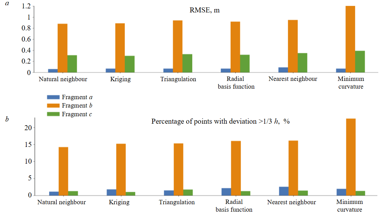
Fig.4. Assessment of the accuracy of methods for constructing DEM on the assigned fragments
Checking the accuracy of DEM constructed using spatial interpolation methods for the entire project
Construction and accuracy assessment of digital elevation models created for the entire area of plots A, B and C were accomplished. Thus, the results obtained at the previous stage are aimed at getting a preliminary idea of the accuracy of DEM produced for each plot of the earth's surface, since differences in topography types clearly indicate the need to use a differentiated approach. Histogram with estimated parameters for fragments a, b and c is shown in Fig.4. A comprehensive assessment of the accuracy of constructed models for plots A, B and C is given in Table 7.
<з class="text">Table 7
Assessment of the accuracy of digital elevation models
|
Method |
RMSE of height |
Number of points |
Percentage of points deviating by more |
Percentage of points deviating by more than h, m |
|
Flat plot A |
||||
|
Natural neighbour |
0.11 |
53,288,238 |
5.84 |
0.84 |
|
Kriging |
0.12 |
53,288,238 |
6.78 |
1.06 |
|
Triangulation with linear interpolation |
0.12 |
53,288,238 |
6.93 |
1.09 |
|
Mountainous plot B with anthropogenic topography |
||||
|
Kriging |
0.55 |
4,556,172 |
6.63 |
0.77 |
|
Natural neighbour |
0.57 |
4,556,172 |
7.17 |
0.80 |
|
Radial basis function |
0.57 |
4,556,172 |
7.08 |
0.95 |
|
Mountainous plot C |
||||
|
Kriging |
0.29 |
17,476,315 |
0.83 |
0.01 |
|
Natural neighbour |
0.29 |
17,476,315 |
0.91 |
0.01 |
|
Radial basis function |
0.29 |
17,476,315 |
0.94 |
0.01 |
Methods of spatial interpolation according to the considered plots should be noted:
- Natural neighbour for plot A. Consistent with assessment of the accuracy of the characteristic fragment.
- Quadric kriging with a variogram component according to the Gaussian (normal) distribution and a natural neighbour for plot B. Partially consistent with assessment of the accuracy of the characteristic fragment. Differences in the comprehensive assessment appeared to be negligible, since the natural neighbour method showed greater resistance to the formation of outliers in the topographic surface. The kriging method slightly surpassed the natural neighbour method by other estimated parameters.
- Quadric kriging with a spherical variogram component for plot C. Consistent with a comprehensive assessment of the accuracy of the characteristic fragment.
Conclusion
In hard-to-reach regions, development or assessment of the integrity of the existing elevation datum is problematic. Creation of digital models will significantly reduce the production costs for repeated measurements of the investigated plots and search for the most productive solutions on choosing an algorithm for constructing a mathematical analogue with pre-assigned accuracy. Reducing the costs of constructing digital models will increase the availability of a single set of reliable geospatial information, which is used in designing, construction and further monitoring of buildings and engineering structures, in assessing the risk of landslides, flood monitoring and is the basis for research in Earth sciences based on background information.
Investigation of the accuracy of the local quasigeoid model showed:
- The least RMSE interpolation value for an area project was attained using triangulation with linear interpolation (0.003 m) and kriging (0.003 m). The least RMSE value for determining the heights by control points for an area project was obtained using the natural neighbour (0.004 m) and kriging (0.004 m) methods.
- The least RMSE for determining the heights from the model was shown by kriging (0.006 m) and triangulation with linear interpolation (0.006 m). When assessing the accuracy of constructing a model on control points, the least RMSE value for determining the heights was obtained using the kriging method (0.007 m).
- When constructing quasigeoid models, it is necessary to determine the number of starting points in the work area, which depends on anomality of the region. When designing the required number of points in a given area, the recommended spacing between combined points is 5 km.
Investigation of DEM construction accuracy showed:
- Construction of a digital elevation model applying the natural neighbour method on flat plot A of the earth’s surface led to the least aggregate value of the estimated parameters: RMSE, “Percentage of points deviating by more than 0.33 m”, and “Percentage of points deviating by more than 5 m”.
- For DEM construction on mountainous plot B on the earth’s surface with pronounced anthropogenic topography, the authors proposed the quadric kriging method with a variogram component according to the Gaussian (normal) distribution.
- For mountainous plot C, the authors identified the quadric kriging method with a spherical variogram component based on the least values of the estimated parameters.
- The approach to assessing the accuracy of construction based on the characteristic flat and mountainous fragments turned out to be efficient, since it was confirmed when constructing a DEM for the entire flat and mountainous project site. This is due to similar morphometric characteristics. On the mountainous fragment with anthropogenic topography such approach requires additional control by two spatial interpolation methods that are close to the optimal one in terms of the estimated parameters, which is accounted for by areas with a marked change in surface curvature;
All spatial interpolation methods resulted in deviations above the permissible ones for topographic surfaces on flat, mountainous plots with anthropogenic topography, and mountainous plots of the earth’s surface with the least percentage deviations of 5.84, 6.63, and 0.83 %, respectively.
References
- Ponomarenko M.R., Kutepov Yu.I., Shabarov A.N. Open pit mining monitoring support with information and analysis using web mapping technologies. Mining Informational and Analytical Bulletin. 2022. N 8, p. 56-70 (in Russian). DOI: 10.25018/0236_1493_2022_8_0_56
- Raguzin I.I., Bykova E.N., Lepikhina O.Yu. Polygonal Metric Grid Method for Estimating the Cadastral Value of Land Plots. Lomonosov Geography Journal. 2023. Vol. 78. N 3, p. 92-103 (in Russian). DOI: 10.55959/MSU0579-9414.5.78.3.8
- Bykowa E., Skachkova M., Raguzin I. et al. Automation of Negative Infrastructural Externalities Assessment Methods to Determine the Cost of Land Resources Based on the Development of a “Thin Client” Model. Sustainability. 2022. Vol. 14. Iss. 15. N 9383. DOI: 10.3390/su14159383
- Bazhin V.Yu., Masko O.N., Martynov S.A. Automatic burden balance monitoring and control in the production of metallurgical silicon. Tsvetnye metally. 2023. N 4, p. 53-60 (in Russian). DOI: 10.17580/tsm.2023.04.07
- Bazhin V.Yu., Masko O.N., Huy H. Nguyen. Increasing the speed of information transfer and operational decision-making in metallurgical industry through an industrial bot. Non-ferrous Metals. 2023. N 1, p. 62-67. DOI: 10.17580/nfm.2023.01.10
- Gendler S.G., Kryukova M.S. Thermal management of metro lines, including double-track and single-track tunnels. Mining Informational and Analytical Bulletin. 2023. N 9-1, p. 248-269 (in Russian). DOI: 10.25018/0236_1493_2023_91_0_248
- Karasev М.А., Pospehov G.B., Astapenko T.S., Shishkina V.S. Stress–strain behavior prediction models for weak manmade soil. Mining Informational and Analytical Bulletin. 2023. N 11, p. 49-69 (in Russian). DOI: 10.25018/0236_1493_2023_11_0_49
- Kulchitskiy A.A., Mansurova O.K., Nikolaev M.Yu. Recognition of defects in hoisting ropes of metallurgical equipment by an optical method using neural networks. Chernye metally. 2023. N 3, р. 81-88 (in Russian). DOI: 10.17580/chm.2023.03.13
- Petrov P.A., Shestakov A.K., Nikolaev M.Yu. Use of multifunctional crust breaker and machine vision system for acquisition and processing of aluminium reduction cell data. Tsvetnye metally. 2023. N 4, p. 45-53 (in Russian). DOI: 10.17580/tsm.2023.04.06
- Petrova T.A., Astapenko T.S., Kalahryuka A.A., Yesman M.M. Reducing the geo-environmental impact of halite waste storage. Mining Informational and Analytical Bulletin. 2022. N 10-1, p. 155-162. DOI: 10.25018/0236_1493_2022_101_0_155
- Belikov A.A., Belyakov N.A. Method of predicting the stress-strain state of interchamber pillars lined with a compliant rope fastener. Mining Informational and Analytical Bulletin. 2023. N 4, p. 20-34 (in Russian). DOI: 10.25018/0236_1493_2023_4_0_20
- Belyakov N.A., Belikov A.A. Prediction of the integrity of the water-protective stratum at the Verkhnekamskoye potash ore deposit. Mining Informational and Analytical Bulletin. 2022. N 6-2, p. 33-46 (in Russian). DOI: 10.25018/0236_1493_2022_62_0_33
- Huxiong Li, Weiya Ye, Jun Liu et al. High-Resolution Terrain Modeling Using Airborne LiDAR Data with Transfer Learning. Remote Sensing. 2021. Vol. 13. Iss. 17. N 3448. DOI: 10.3390/rs13173448
- Hashemi-Beni L., Jones J., Thompson G. et al. Challenges and Opportunities for UAV-Based Digital Elevation Model Generation for Flood-Risk Management: A Case of Princeville, North Carolina. Sensors. 2018. Vol. 18. Iss. 11. N 3843. DOI: 10.3390/s18113843
- Gusev V.N., Blishchenko A.A., Sannikova A.P. Study of a set of factors influencing the error of surveying mine facilities using a geodetic quadcopter. Journal of Mining Institute. 2022. Vol. 254, p. 173-179. DOI: 10.31897/PMI.2022.35
- Kremcheev E.A., Danilov A.S., Smirnov Yu.D. Metrological Support of Monitoring Systems Based on Unmanned Aerial Vehicles. Journal of Mining Institute. 2019. Vol. 235, p. 96-105. DOI: 10.31897/PMI.2019.1.96
- Menshikov S.N., Dzhaljabov A.A., Vasilev G.G. et al. Spatial Models Developed Using Laser Scanning at Gas Condensate Fields in the Northern Construction-Climatic Zone. Journal of Mining Institute. 2019. Vol. 238, p. 430-437. DOI: 10.31897/PMI.2019.4.430
- Luethje F., Tiede D., Eisank C. Terrain Extraction in Built-Up Areas from Satellite Stereo-Imagery-Derived Surface Models: A Stratified Object-Based Approach. ISPRS International Journal of Geo-Information. 2017. Vol. 6. Iss. 1. N 9.DOI: 10.3390/ijgi6010009
- Das R.K., Samanta S., Jana S.K., Rosa R. Polynomial interpolation methods in development of local geoid model. The Egyptian Journal of Remote Sensing and Space Science. 2018. Vol. 21. Iss. 3, p. 265-271. DOI: 10.1016/j.ejrs.2017.03.002
- Ahmed H.M., Mohamed E.A., Bahaa S.A. Evaluating two numerical methods for developing a local geoid model and a local digital elevation model for the Red Sea Coast, Egypt. Journal of King Saud University – Engineering Sciences. 2023. Vol. 35. Iss. 6, p. 384-392. DOI: 10.1016/j.jksues.2021.04.004
- Banasik P., Bujakowski K. The Use of Quasigeoid in Leveling Through Terrain Obstacles. Reports on Geodesy and Geoinformatics. 2017. Vol. 104. Iss. 1, p. 57-64. DOI: 10.1515/rgg-2017-0015
- Borowski Ł., Banaś M. The Best Robust Estimation Method to Determine Local Surface. Baltic Journal of Modern Computing. 2019. Vol. 7. N 4, p. 525-540. DOI: 10.22364/bjmc.2019.7.4.06
- Habib M., Alzubi Y., Malkawi A., Awwad M. Impact of interpolation techniques on the accuracy of large-scale digital elevation model. Open Geosciences. 2020. Vol. 12. Iss. 1, p. 190-202. DOI: 10.1515/geo-2020-0012
- Amodio A.M., Aucelli P.P.C., Garfì V., Rosskopf C.M. Digital photogrammetric analysis approaches for the realization of detailed terrain models. Rendiconti Online della Società Geologica Italiana. 2020. Vol. 52, p. 69-75. DOI: 10.3301/ROL.2020.21
- Bui L.K., Glennie C.L., Hartzell P.J. Rigorous Propagation of LiDAR Point Cloud Uncertainties to Spatially Regular Grids by a TIN Linear Interpolation. IEEE Geoscience and Remote Sensing Letters. 2022. Vol. 19. N 7003105. DOI: 10.1109/LGRS.2021.3134587
- Boreggio M., Bernard M., Gregoretti C. Evaluating the Differences of Gridding Techniques for Digital Elevation Models Generation and Their Influence on the Modeling of Stony Debris Flows Routing: A Case Study From Rovina di Cancia Basin (North-Eastern Italian Alps). Frontiers in Earth Science. 2018. Vol. 6. N 89. DOI: 10.3389/feart.2018.00089
- Fazilova D., Magdiev H. Comparative Study of Interpolation Methods in Development of Local Geoid. International Journal of Geoinformatics. 2018. Vol. 14. N 1, p. 29-33.
- Banasik P., Bujakowski K., Kudrys J. et al. Development of a precise local quasigeoid model for the city of Krakow – QuasigeoidKR2019. Reports on Geodesy and Geoinformatics. 2020. Vol. 109. Iss. 1, p. 25-31. DOI: 10.2478/rgg-2020-0004
- Mysen E. On the uncertainty of height anomaly differences predicted by least-squares collocation. Journal of Geodetic Science. 2020. Vol. 10. Iss. 1, p. 53-61. DOI: 10.1515/jogs-2020-0111
- Hosseini-Asl M., Amiri-Simkooei A.R., Safari A. Establishment of a corrective geoid surface by spline approximation of Iranian GNSS/levelling network. Measurement. 2022. Vol. 197. N 111341. DOI: 10.1016/j.measurement.2022.111341
- Medved K., Kuhar M., Koler B. Regional gravimetric survey of central Slovenia. Measurement. 2019. Vol. 136, p. 395-404. DOI: 10.1016/j.measurement.2018.12.065
- Chymyrov A. Comparison of different DEMs for hydrological studies in the mountainous areas. The Egyptian Journal of Remote Sensing and Space Science. 2021. Vol. 24. Iss. 3. Part 2, p. 587-594. DOI: 10.1016/j.ejrs.2021.08.001
- Mahbuby H., Safari A., Foroughi I. Local gravity field modeling using spherical radial basis functions and a genetic algorithm. Comptes Rendus Geoscience. 2017. Vol. 349. N 3, p. 106-113. DOI: 10.1016/j.crte.2017.03.001
- Belay E.Y., Godah W., Szelachowska M., Tenzer R. ETH-GQS: An estimation of geoid-to-quasigeoid separation over Ethiopia. Geodesy and Geodynamics. 2022. Vol. 13. Iss. 1, p. 31-37. DOI: 10.1016/j.geog.2021.09.006
- Qingwang Liu, Liyong Fu, Qiao Chen et al. Analysis of the Spatial Differences in Canopy Height Models from UAV LiDAR and Photogrammetry. Remote Sensing. 2020. Vol. 12. Iss. 18. № 2884. DOI: 10.3390/rs12182884
- Mustafin M.G., Balandin V.N., Bryn M.Ja. et al. Topographic-geodetic and Cartographic Support of the Arctic Zone of the Russian Federation. Journal of Mining Institute. 2018. Vol. 232, p. 375-382. DOI: 10.31897/PMI.2018.4.375
- Mustafin M.G., Valkov V.A., Kazantsev A.I. Monitoring of Deformation Processes in Buildings and Structures in Metropolises. Procedia Engineering. 2017. Vol. 189, p. 729-736. DOI: 10.1016/j.proeng.2017.05.115
- Rusli N., Majid M.R., Nur Fakihin Auni A. Razali, Nur Fatma Fadilah Yaacob. Accuracy Assessment of DEM from UAV and TanDEM-X Imagery. 2019 IEEE 15th International Colloquium on Signal Processing & Its Applications, 8-9 March 2019, Penang, Malaysia. IEEE Xplore, 2019, p. 127-131. DOI: 10.1109/CSPA.2019.8696088
- Habib M. Evaluation of DEM interpolation techniques for characterizing terrain roughness. Catena. 2021. Vol. 198. N 105072. DOI: 10.1016/j.catena.2020.105072
- Li L., Nearing M.A., Nichols M.H. et al. The effects of DEM interpolation on quantifying soil surface roughness using terrestrial LiDAR. Soil and Tillage Research. 2020. Vol. 198. N 104520. DOI: 10.1016/j.still.2019.104520
- Chuanfa Chen, Yixuan Bei, Yanyan Li, Weiwei Zhou. Effect of interpolation methods on quantifying terrain surface roughness under different data densities. Geomorphology. 2022. Vol. 417. N 108448. DOI: 10.1016/j.geomorph.2022.108448
- Cățeanu M., Ciubotaru A. Accuracy of Ground Surface Interpolation from Airborne Laser Scanning (ALS) Data in Dense Forest Cover. ISPRS International Journal of Geo-Information. 2020. Vol. 9. Iss. 4. N 224. DOI: 10.3390/ijgi9040224
- Tao Zhang, Xiaosu Xu, Shengbao Xu. Method of establishing an underwater digital elevation terrain based on kriging interpolation. Measurement. 2015. Vol. 63, p. 287-298. DOI: 10.1016/j.measurement.2014.12.025
- Ikechukwu M.N., Ebinne E., Idorenyin U., Raphael N.I. Accuracy Assessment and Comparative Analysis of IDW, Spline and Kriging in Spatial Interpolation of Landform (Topography): An Experimental Study. Journal of Geographic Information System. 2017. Vol. 9. N 3, p. 354-371. DOI: 10.4236/jgis.2017.93022
- Pavlova A.I. Analysis of elevation interpolation methods for creating digital elevation models. Optoelectronics, Instrumentation and Data Processing. 2017. Vol. 53. N 2, p. 171-177. DOI: 10.3103/S8756699017020108
- Helwig Z.D., Guggenberger J., Elmore A.C., Uetrecht R. Development of a variogram procedure to identify spatial outliers using a supplemental digital elevation model. Journal of Hydrology X. 2019. Vol. 3. N 100029. DOI: 10.1016/j.hydroa.2019.100029
- Arun P.V. A comparative analysis of different DEM interpolation methods. The Egyptian Journal of Remote Sensing and Space Science. 2013. Vol. 16. Iss. 2, p. 133-139. DOI: 10.1016/j.ejrs.2013.09.001
- Bui L.K., Glennie C.L. Estimation of lidar-based gridded DEM uncertainty with varying terrain roughness and point density. ISPRS Open Journal of Photogrammetry and Remote Sensing. 2023. Vol. 7. N 100028. DOI: 10.1016/j.ophoto.2022.100028
- Agüera-Vega F., Agüera-Puntas M., Martínez-Carricondo P. et al. Effects of point cloud density, interpolation method and grid size on derived Digital Terrain Model accuracy at micro topography level. International Journal of Remote Sensing. 2020. Vol. 41. Iss. 21, p. 8281-8299. DOI: 10.1080/01431161.2020.1771788
- McRoberts R.E., Domke G.M., Qi Chen et al. Using genetic algorithms to optimize k-Nearest Neighbors configurations for use with airborne laser scanning data. Remote Sensing of Environment. 2016. Vol. 184, p. 387-395. DOI: 10.1016/j.rse.2016.07.007