
Modelling of compositional gradient for reservoir fluid in a gas condensate deposit with account for scattered liquid hydrocarbons
- 1 — Junior Researcher Oil and Gas Research Institute of RAS ▪ Orcid
- 2 — Ph.D., Dr.Sci. Deputy Director for Research Oil and Gas Research Institute of RAS ▪ Orcid
- 3 — Ph.D. Senior Researcher Oil and Gas Research Institute of RAS ▪ Orcid ▪ Scopus
- 4 — Senior Researcher Oil and Gas Research Institute of RAS ▪ Orcid
- 5 — Ph.D., Dr.Sci. Professor Peoples’s Friendship University of Russia named after Patrice Lumumba ▪ Orcid
Abstract
In oil and gas reservoirs with significant hydrocarbon columns the dependency of the initial hydrocarbon composition on depth – the compositional gradient – is an important factor in assessing the initial amounts of components in place, the position of the gas-oil contact, and variations of fluid properties throughout the reservoir volume. Known models of the compositional gradient are based on thermodynamic relations assuming a quasi-equilibrium state of a multi-component hydrodynamically connected hydrocarbon system in the gravity field, taking into account the influence of the natural geothermal gradient. The corresponding algorithms allow for calculation of changes in pressure and hydrocarbon fluid composition with depth, including determination of the gas-oil contact (GOC) position. Above and below the GOC, the fluid state is considered single-phase. Many oil-gas-condensate reservoirs typically have a small initial fraction of the liquid hydrocarbon phase (LHC) – scattered oil – within the gas-saturated part of the reservoir. To account for this phenomenon, a special modification of the thermodynamic model has been proposed, and an algorithm for calculating the compositional gradient in a gas condensate reservoir with the presence of LHC has been implemented. Simulation cases modelling the characteristic compositions and conditions of three real oil-gas-condensate fields are considered. The results of the calculations using the proposed algorithm show peculiarities of variations of the LHC content and its impact on the distribution of gas condensate mixture composition with depth. The presence of LHC leads to an increase in the level and possible change in the type of the fluid contact. The character of the LHC fraction dependency on depth can be different and is governed by the dissolution of light components in the saturated liquid phase. The composition of the LHC in the gas condensate part of the reservoir changes with depth differently than in the oil zone, where the liquid phase is undersaturated with light hydrocarbons. The results of the study are significant for assessing initial amounts of hydrocarbon components and potential efficiency of their recovery in gas condensate and oil-gas-condensate reservoirs with large hydrocarbon columns.
The study was fulfilled in the framework of OGRI RAS state assignment, topics 122022800272-4 “Improving the methods of modelling, laboratory and field studies for creation of new technologies for efficient environmentally friendly hydrocarbon recovery in complex mining and geological conditions” and 122022800274-8 “Creation of scientific foundations for a new system methodology for forecasting, prospecting and development of hydrocarbon reservoirs, including matrix oil deposits in gas-saturated carbonate deposits of oil-gas-condensate fields”
Introduction
Assessing the distribution of the initial component composition of reservoir fluid within the productive formation is one of the key tasks in the comprehensive reservoir study, evaluation of hydrocarbons in place, and development planning. Actual data for analyzing the spatial variation in composition and properties of hydrocarbons are provided by studies of reservoir fluid samples [1, 2], measurements of flow characteristics by formation testers [3, 4], well tests and gas condensate studies [5, 6], and optical methods [7]. Geochemical studies [8, 9], biomarkers [10, 11], hydrocarbon group and isotopic analysis [12, 13], combined with statistical analysis and clustering methods [14], and thorough analysis of reservoir pressure dynamics for developed objects [15] allow identifying various sources of hydrocarbon fluid influx into the reservoir, while well test studies, interference testing, tracer tests, and analysis of fluid contacts reveal the presence of hydrodynamically disconnected zones within the formation [16-18].
In many reservoirs, a regular change in fluid composition with depth is observed. Most often it manifests as an increase in density and a decrease in solution gas-oil ratio and saturation pressure for oil, or an increase in condensate content and saturation (dew point) pressure for gas condensate system [1, 2, 19]. This phenomenon is referred to as the compositional gradient. Theoretical models of the compositional gradient, calibrated against actual data, are used to calculate the initial content of hydrocarbons in the formation, refine the position of gas-oil contacts, obtain initial data for designing the reservoir development and initializing mathematical models of the formation [1, 20, 21]. Information on variations in composition and phase state of the fluid helps to optimize well operation regimes and production equipment, assess alternative recovery methods and injection agents, considering the dependency of fluid properties and miscibility conditions on depth. Ultimately, these factors can significantly influence the field development strategy from the economic perspective [22, 23].
In the case of oil-gas-condensate reservoirs, existing models of the compositional gradient allow calculating changes in composition and pressure within the gas-saturated and oil-saturated intervals, as well as assessing the position of the gas-oil contact (GOC). However, they do not account for the possible presence of what is known as scattered oil (liquid hydrocarbons – LHC) in the gas condensate part of the reservoir from the beginning of development, confirmed for a number of large oil-gas-condensate fields.
This article presents a modification of the method and algorithm for calculating the compositional gradient, taking into account the presence of LHC in the gas condensate part of the reservoir. It studies the peculiarities of variations in the initial fluid composition and LHC fraction in the gas-saturated interval based on three cases modeling the conditions of real oil-gas-condensate reservoirs.
Methods
Theoretical models of compositional gradient
Compositional gradient models can be categorized into isothermal and those considering the natural temperature (geothermal) gradient.
The relation for calculating the change in fluid composition under the effect of gravity in an isothermal system was first derived by Gibbs [24]. He demonstrated that for a multi-component isothermal system in equilibrium conditions in the gravity field, a balance holds between the change in chemical and gravitational potential with depth. The equilibrium condition is expressed as
where μi is the chemical potential of component i at depth h; Mi is the molar mass of component i; g is the gravity constant (acceleration of gravity); N is the number of components in the system.
By integrating (1) and expressing chemical potentials via fugacities using the equation of state, the relationship can be transformed into a system of algebraic equations for sequential determination of pressure values and component concentrations at different depths with a step Δh [1]. Thus, moving upwards and downwards from a reference point with given fluid composition and pressure allows for calculation of the vertical distributions for pressure and component concentrations. The described procedure is applicable to a single-phase state of the reservoir hydrocarbon system. Features related to determining the position of the GOC are discussed below.
Equation (1) assumes that the system as a whole is at a constant temperature (dT/dh = 0). The isothermal model is applicable to real reservoirs with small depth ranges (hydrocarbon columns) and temperature gradients. In other cases, it is recommended to consider the influence of the geothermal gradient.
In the natural geothermal field, the vertical temperature gradient causes the thermodiffusion effect – an additional “thermal force” that influences the distribution of component concentrations with depth. To quantitatively assess the influence of thermodiffusion, models that consider both gravitational and thermal factors are used. The quasi-equilibrium distribution of composition with depth formed by these factors obeys the following general balance equation [20]
where zi is the component molar fraction; h is the depth; and are the gravity segregation force and the thermal force for component i, respectively.
The main factor controlling the change in composition with depth is usually the gravitational force. Thermodiffusion typically acts against gravity and weakens its influence on the manifestation of the compositional gradient. In most reservoirs, the impact of the thermal force is less than that of the gravity force [20, 25].
One of the most theoretically justified and practically convenient models for the thermal force was proposed by Haase [26, 27]. In this model, the thermal force can be obtained via the limiting values of thermodiffusion coefficients at temperature gradient approaching zero and takes the form:
where are the molecular mass and partial molar enthalpy of component i; M and H are the molecular mass and molar enthalpy of the mixture.
Based on the Haase model, Pedersen and Lindelof derived the following relationship for calculating the compositional gradient [19, 21, 28]:
where p is the pressure; is the vector of molar component concentrations in the mixture (molar composition of the mixture); T1 and T2, h1 and h2 are the values of temperature and depth for the first and second points considered, respectively; R is the universal gas constant; fi is the fugacity of component i.
The dependence of fugacities on pressure and mixture composition is determined by solving the cubic equation of state, for example, the Peng – Robinson equation. The system of equations (2) is solved for pressure and fluid composition at point h2 at each step in depth, given the known values at point h1. Details of the enthalpy calculations are presented in [19, 29].
Practical implementation of the compositional gradient model
In this study, a conservative finite difference scheme [30] is used to implement the compositional gradient model (the problem of compositional grading). To solve the obtained system of nonlinear algebraic equations, Newtonʼs method is applied providing an efficient solution to the compositional grading problems when using the solution from the previous step as the initial approximation [1, 2]. Sequential search for the values of the basic unknowns is performed at each iteration by solving the system of linear equations AY = b using the Gauss elimination method, the choice of which is determined by the dense structure of the matrix and the typical dimensionality of several tens of equations:
where superscript m corresponds to the current, and m – 1 – to the previous iteration; ψi is the misfit of equation (2) for component i at the previous iteration (with opposite sign); Δ is the change in the basic unknown at the current iteration. As the initial approximation at the first iteration, the values at depth h1 are used.
Thus, if the composition and pressure are known at the reference depth, they can be sequentially determined for any other specified depth using the system (2). The temperature values at each depth are considered known according to the specified geothermal gradient. The input data of the model are the parameters of the equation of state and specific enthalpies of the components. For pure substances, these are reference data, while for pseudocomponents and fractions they are determined by using correlations presented in the literature and solving identification problems with actual measurements from the studies of formation fluid samples.
The described model is applicable for a single-phase state of the system. The classical calculation of the compositional gradient assumes that the mixture reaches the saturation point and transitions to the two-phase state at the depth of GOC. To check the phase state of the mixture, a special iterative procedure is used – the Michelsen stability test [31]. Stability obtained in this test indicates the single-phase state of the mixture, while instability indicates the two-phase state corresponding to crossing the GOC. Thus, to search for the GOC, the stability of the mixture is checked for the obtained pressure and composition at each depth. If the mixture becomes unstable at the successive step, a bisection algorithm is implemented within the corresponding depth interval to determine the precise GOC position [32].
At the depth of the GOC, the pressure equals the saturation (dew point) pressure of the gas phase (when approaching from above) and the saturation pressure of the liquid phase (when approaching from below). Therefore, an alternative method for finding the GOC involves calculating the pressure of mixture transition to the two-phase state at each step in depth [33]. Once the GOC position is found, a transition is necessary from the gas phase composition to the equilibrium liquid phase composition, or vice versa. For this, the phase equilibrium problem is solved [1, 2].
These features are valid for the classical (saturated) GOC. In deep formations with high pressures and temperatures, the transition from gas to liquid phase may be supercritical. In this case, a two-phase state within the reservoir does not occur, but the single-phase fluid changes its type from gaseous to liquid at the GOC. At the GOC, the mixture saturation pressure reaches its maximum, which is lower than the pressure at the GOC.
It is important to note the differences between the thermodynamic calculations of the compositional gradient and the principles used in the equilibrium initialization of the flow simulation models for oil and gas reservoirs. In flow simulations, the effects of thermodiffusion are not considered, whereas classical calculations of the compositional gradient do not account for the presence of the gas – oil capillary transition zone. The coexistence of gaseous and liquid hydrocarbon phases is assumed at the GOC only.
The gas – oil transition zone is usually limited to few, rarer first tens of meters, which is due to greater difference in phase densities and lower values of surface tension than for the oil – water system. Whereas the effect of the compositional gradient manifests itself over larger depth ranges, measured by hundreds of meters. At the same time, the influence of capillary pressure on the gas – oil phase equilibria is not significant even in tight reservoirs [1, 22], and has a noticeable effect only in shale reservoirs. Thus, it is assumed that neglecting the influence of capillary pressure and the presence of the two-phase gas – oil transition zone does not significantly affect the calculation of the initial hydrocarbon composition distribution with depth. In this study, the authors also follow this approach and do not account for the presence of the gas – oil capillary transition zone. The possibility to overcome this limitation is discussed in the conclusions.
Compositional gradient in the presence of scattered liquid hydrocarbon phase
In gas condensate reservoirs, the presence in the pores of a small volume of immobile LHC is often reported, referred to as scattered, relict, residual, or matrix oil [1, 34]. In this case, the described classical calculation of quasi-equilibrium initial fluid distribution is not applicable, as it assumes the coexistence of two phases at the GOC only [22].
The presence of such fluid type in the gas condensate part of the reservoir was first identified for the Orenburg oil-gas-condensate field (OGCF) both by core data and phase behavior characteristics of the fluid [1, 35]. The presence of LHC in gas-saturated intervals has been confirmed for the main reservoir of the Vuktyl OGCF [34] and is probably characteristic for other OGCFs [22]. Unlike condensate, LHC is present in the gas-saturated zone of the formation from the beginning of development and is distinguished by heavier composition, including resins and asphaltenes. The presence of LHC is noted throughout the depth interval of the gas-saturated zone, not just in the relatively small capillary transition zone near the GOC. The saturation for scattered LHC is usually estimated at 5-15 %.
Studies [34, 35] offered the following explanation for this phenomenon. The terms “matrix oil” and “LHC” in this context correspond to the paradigm of oil-gas source properties of hydrocarbon bearing carbonate deposits that form gas condensate and oil-gas-condensate fields, in particular, the Vuktyl and Orenburg fields. The presence of inherent (matrix) oil, transformed into liquid hydrocarbons of the oil sequence (LHC), in the pore space of the carbonate rocks of the gas part of these fields has been demonstrated as a result of previous studies. The established oil-gas source properties and early stages of oil generation in hydrocarbon bearing deposits allow for the assertion that even before the start of development LHC are present in their gas part in thermodynamic equilibrium with gas, but at saturations below the critical values (flow threshold). These are the LHC considered in this study.
To account for LHC in the gas condensate part of the reservoir, a modified algorithm for the compositional gradient was proposed in [36]. It assumes that the gas phase is continuously connected through depth and its composition corresponds to the quasi-equilibrium conditions (2). The liquid phase is immobile and not connected between depths, so the quasi-equilibrium conditions for the liquid phase are not satisfied. However, at each depth, the liquid phase is in equilibrium with the corresponding composition of the gas phase.
As in the classical calculation, the initial data for the modified algorithm include the fluid composition at the reference depth, pressure, temperature, and the geothermal gradient. Due to the presence of LHC, the overall composition of the fluid at the reference depth must correspond to a two-phase state with a fraction of the liquid hydrocarbon phase estimated from well logging and core analysis. For this purpose, the composition of the gas condensate fluid obtained from samples is preliminarily saturated to the corresponding molar fraction of LHC L0 [22].
This saturation procedure is necessary for the following reason. Due to the presence of LHC in the gas condensate part of the reservoir, any change in reservoir pressure near the well converts the system into the two-phase state associated not only with condensate dropout but also with gas liberation from the saturated oil (LHC). This leads to some distortion of the fluid composition during standard procedures of gas condensate tests. As a result, the fluid sample may become undersaturated, which prevents using its composition as that of the reservoir gas condensate mixture in the presence of LHC. For example, in the case of the Vuktyl OGCF, the difference between the reservoir pressure and the saturation pressure by samples ranges from 20 to 40 bar and increases with depth [34].
Thus, unlike the classical compositional gradient, the input composition in the algorithm with LHC at the reference depth is set to be unstable. This is controlled by the Michelsen stability test [31]. The next step is to determine the corresponding equilibrium compositions of the gas (vapor) and liquid phases, as well as the calculated fraction of LHC by solving the phase equilibrium problem [2]. The calculated LHC fraction must match the value L0. The obtained gas phase composition is saturated and is further used as the input mixture composition for calculating the compositional gradient upwards and downwards from the reference point.
When moving downwards, the composition of the gas condensate mixture becomes heavier (richer). The gas phase, saturated at the previous step, becomes oversaturated at the new point, i.e., transforms into a two-phase mixture . For this mixture, at the pressure and temperature of the new depth, the equilibrium compositions of the gas phase and liquid phase , and their fractions Vh = 1 – Lh and Lh are determined. The resulting gas phase again becomes saturated.
When moving upwards, the composition of the gas condensate mixture becomes lighter (leaner), so the mixture becomes undersaturated. A pseudoequilibrium liquid phase composition can be calculated for the mixture using the Negative Flash procedure proposed by Whitson and Michelsen [37].
The Negative Flash extends the standard phase equilibrium algorithm beyond the two-phase region to enable calculations when the fluid is single-phase. The value of the gas phase molar fraction 0 < Vh < 1, both in the standard phase equilibrium calculation and in the Negative Flash, implies that Vh moles of gas of the calculated composition need to be added to 1 – Vh moles of liquid of the calculated composition to restore the original mixture composition . Similarly, Vh > 1 (undersaturated gas) in the Negative Flash procedure is interpreted as the Vh – 1 moles of liquid with composition need to be removed from Vh moles of gas of composition to restore one mole of the original mixture .
Thus, in the both cases (steps upwards and downwards), the saturated gas phase composition obtained as a result of the Negative Flash procedure is taken as the final composition of the gas condensate mixture at the new depth, and the composition of the liquid phase is considered the equilibrium LHC composition at that depth. The LHC fraction is adjusted compared to the value at the previous depth, taking into account additional condensation from the gas condensate mixture upon oversaturation (step downwards) or, conversely, evaporation upon undersaturation (step upwards):
where Li is the final LHC fraction at the new depth; Lh is the LHC fraction obtained from the Negative Flash procedure.
During the movement downwards in the algorithm with LHC, reaching the GOC is controlled with L1 = 1 (transition to the single-phase liquid state). When moving upwards, the possible transition to the single-phase gas state (L1 = 0) is controlled. In both the cases, further steps are carried out using the classical (single-phase) calculation of the compositional gradient.
The overall flowchart of the algorithm considering LHC is presented in Fig.1.
Discussion of results
Evaluation of the impact of LHC on the composition distribution in gas condensate reservoirs
The described algorithms for compositional grading were used for computational assessment of the impact of LHC on the distribution of pressure and composition in gas condensate reservoirs. The parameters of multi-component fluid models, reservoir conditions, and initial data at reference depth were taken close to characteristics of three different gas condensate reservoirs: one of the Achimov reservoirs of the Urengoy OGCF, the main reservoir of the Orenburg OGCF, and the main reservoir of the Vuktyl OGCF.
According to core data, the hydrocarbon bearing carbonate oil-gas source rocks of large OGCFs (Vuktyl and Orenburg) before the start of the development are difobic [35], i.e., they express phobicity to water and to a lesser extent to liquid hydrocarbons, with the contact angle of 110-120°. Considering the significant hydrocarbon columns of the studied reservoirs, this becomes an additional factor to consider the size of the transition zone and the influence of capillary forces to be insignificant for this study.
The calculations performed do not account for the entire specificity of the chosen reservoirs and investigate the features of the LHC influence only within the assumptions of the model. For instance, direct studies for the Orenburg OGCF showed the presence of a significant fraction of heavy bitumoids (heavy resins and asphaltenes) in the formation [35]. In the problem formulation considered, their presence and interaction with the modeled reservoir fluid is not accounted for, despite their high adsorption capacity towards light hydrocarbon components. Furthermore, the increased concentrations of heavy bitumoids due to the oil-source properties of the carbonate rocks of the Orenburg OGCF are generally associated with low-permeability hydrophilic intervals with high gas-water capillary pressures, which can have a peculiar “block” effect for the gas phase. The assessment of the influence of these and other additional factors extends beyond the scope of the current stage of the research.
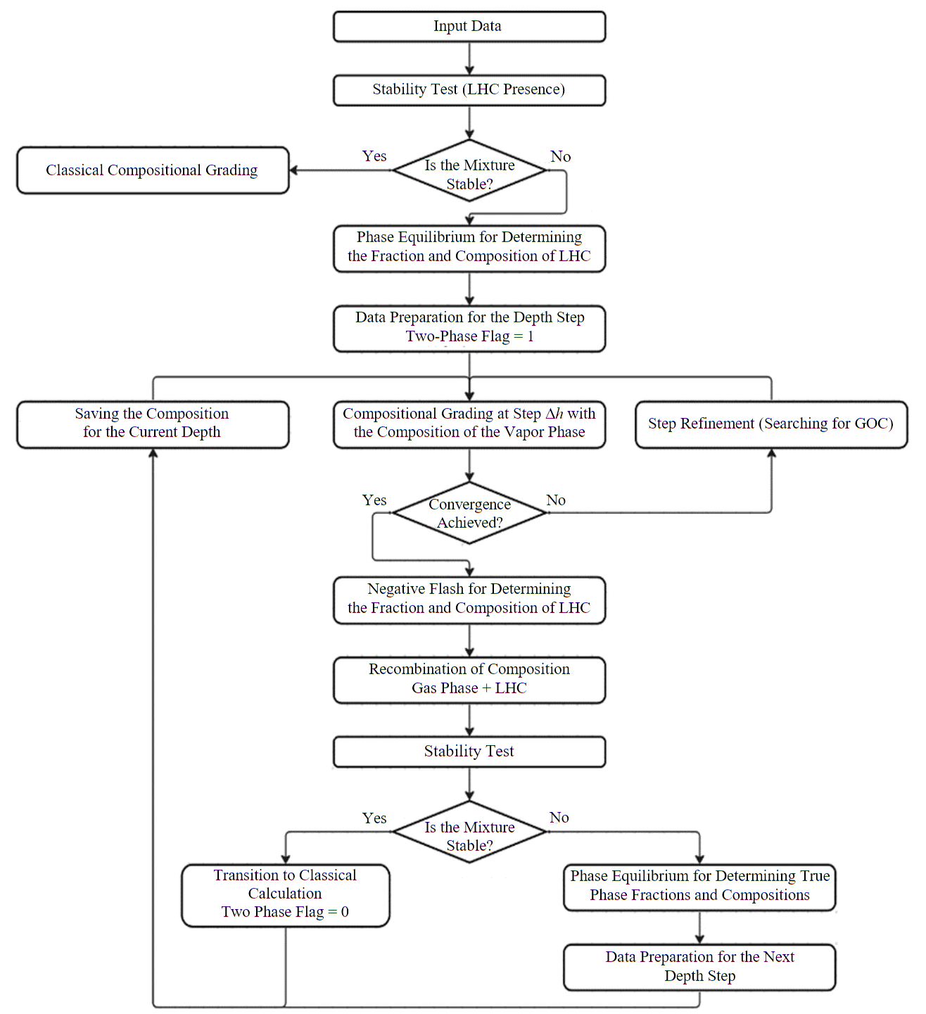
Fig.1. Flowchart of the compositional grading algorithm considering LHC
Composition 1 closely resembles the conditions of one of the Achimov reservoirs of the Urengoy OGCF with a unique condensate content of the reservoir gas. The reservoir fluid is modeled by a mixture of 24 components (Table 1). The reference depth is h = 3754.6 m, pressure at the refe-rence depth is p = 633 bar, temperature is T = 107.85 °C, and the geothermal gradient is dT = = 0.029 °C/m. The composition corresponds to a sample of gas condensate fluid at this depth. The calculation was performed in the depth range of 3614 to 4050 m with the 1 m step.
Table 1
Input data for composition 1
|
Components |
Molar fraction z, % |
Molar mass M, g/mol |
Critical temperature Tc, °С |
Critical pressure pc, bar |
Acentric factor ω |
Molar enthalpy*Href, J |
Coefficients of cubic approximation for ideal gas heat capacity **[38] |
|||
|
A |
B |
C |
D |
|||||||
|
N2 |
0.247 |
28.013 |
–146.95 |
33.9439 |
0.04 |
8330.789 |
31.1488 |
-0.0136 |
0.0 |
0.0 |
|
CO2 |
0.631 |
44.01 |
31.55 |
73.8659 |
0.225 |
19459.1011 |
19.7946 |
0.0734 |
–0.0001 |
0.0 |
|
C1 |
75.2122 |
16.043 |
–82.55 |
46.0421 |
0.013 |
2.6425 |
19.2503 |
0.0521 |
0.0 |
0.0 |
|
C2 |
7.2009 |
30.07 |
32.28 |
48.8387 |
0.0986 |
9761.1347 |
5.4092 |
0.1781 |
–0.0001 |
0.0 |
|
C3 |
4.394 |
44.097 |
96.65 |
42.4552 |
0.1524 |
19519.6224 |
–4.2244 |
0.3063 |
–0.0002 |
0.0 |
|
iC4 |
0.953 |
58.124 |
134.95 |
36.477 |
0.1848 |
29278.1232 |
–1.39 |
0.3847 |
–0.0002 |
0.0 |
|
nC4 |
1.514 |
58.124 |
152.05 |
37.9665 |
0.201 |
29278.1212 |
9.487 |
0.3313 |
–0.0001 |
0.0 |
|
iC5 |
0.537 |
72.151 |
187.25 |
33.8932 |
0.227 |
39036.6099 |
–9.5247 |
0.5066 |
–0.0003 |
0.0 |
|
nC5 |
0.565 |
72.151 |
196.45 |
33.7007 |
0.251 |
39036.6099 |
–3.6257 |
0.4873 |
–0.0003 |
0.0 |
|
C6 |
0.772 |
78.93 |
245.97 |
34.7 |
0.243 |
48795.1026 |
–4.4128 |
0.5819 |
–0.0003 |
0.0 |
|
C7 |
1.16 |
91.8 |
265.95 |
32.5 |
0.292 |
52706.294 |
–5.7687 |
0.5393 |
–0.0002 |
0.0 |
|
C8 |
1.33 |
103.35 |
295.077 |
29.928 |
0.34 |
60741.5508 |
–4.0418 |
0.5889 |
–0.0002 |
0.0 |
|
C9 |
0.801 |
119.17 |
322.415 |
27.987 |
0.388 |
71747.4235 |
–3.2364 |
0.6745 |
–0.0003 |
0.0 |
|
C10 |
0.698 |
133.0 |
346.673 |
26.238 |
0.435 |
81368.8653 |
–0.7145 |
0.7468 |
–0.0003 |
0.0 |
|
C11+ |
0.853 |
153.1083 |
377.537 |
24.1149 |
0.4991 |
63652.7132 |
27.5423 |
0.9068 |
–0.0004 |
0.0 |
|
C13+ |
0.659 |
180.4253 |
415.592 |
21.9509 |
0.5828 |
75009.3798 |
32.4562 |
1.0686 |
–0.0004 |
0.0 |
|
C15+ |
0.542 |
206.7519 |
447.928 |
20.3132 |
0.6605 |
85954.3171 |
37.1921 |
1.2246 |
–0.0005 |
0.0 |
|
C17+ |
0.544 |
237.3727 |
479.571 |
18.6716 |
0.7466 |
98684.4935 |
42.7004 |
1.4059 |
–0.0005 |
0.0 |
|
C20+ |
0.386 |
273.544 |
511.485 |
17.0456 |
0.8454 |
113722.2268 |
49.2071 |
1.6202 |
–0.0006 |
0.0 |
|
C22+ |
0.278 |
308.9098 |
539.266 |
15.7848 |
0.9382 |
128425.0729 |
55.569 |
1.8296 |
–0.0007 |
0.0 |
|
C25+ |
0.206 |
341.7057 |
561.92 |
14.7838 |
1.0222 |
142059.533 |
61.4685 |
2.0239 |
–0.0008 |
0.0 |
|
C27+ |
0.152 |
373.5677 |
581.777 |
13.9428 |
1.1019 |
155305.7262 |
67.2001 |
2.2126 |
–0.0009 |
0.0 |
|
C30+ |
0.137 |
408.5766 |
601.806 |
13.1577 |
1.1878 |
169860.2063 |
73.4978 |
2.42 |
–0.0009 |
0.0 |
|
C36+ |
0.228 |
650.0 |
630.02 |
12.2 |
1.5 |
270228.725 |
116.9268 |
3.8499 |
–0.0015 |
0.0 |
* Partial molar enthalpy in the ideal gas state at 273.15 K, J.
** Coefficients A, B, C, and D are used in enthalpy calculations.
Figure 2 presents the results of the classical algorithm (not considering LHC). PC5+ denotes the potential content of the C5+ component group in the reservoir gas condensate mixture characterizing the amount of dissolved hydrocarbons that exist in liquid state (condensate) in normal conditions [1]. Figure 2 shows that pressure and PC5+ increase with depth (Fig.2, a, b), while the concentration decreases for light components (Fig.2, c) and increases for heavy ones (Fig.2, d, e).
The considered gas condensate reservoir is characterized by near-critical reservoir conditions. Therefore, in Fig.2, a the pressure and saturation pressure at its peak point (GOC) do not match, and a continuous supercritical transition from the gas phase to the liquid phase is seen on the PC5+ curve (Fig.2, b).
To demonstrate the impact of LHC on the component distribution, the mixture composition at the reference point is modified. Pseudo-equilibrium liquid phase with the composition obtained from the Negative Flash procedure is added to the original composition from Table 1, until achieving the LHC molar fraction of 3 % (L0 = 0.03). The results of the calculations using the modified compositional grading algorithm (considering LHC) are shown in Fig.3.
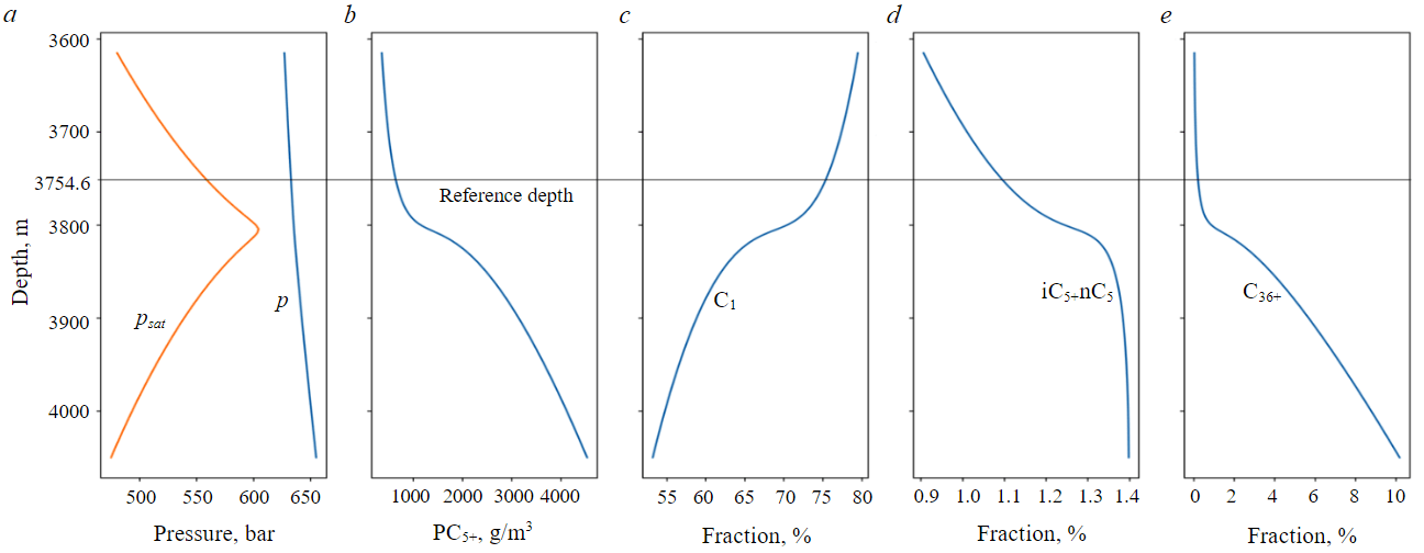
Fig.2. Results of the classical algorithm for composition 1 Calculated dependencies on depth for: a – pressure p and saturation pressure psat, bar; b – PC5+, g/m3; c – molar fraction of methane, %; d – molar fraction of pentanes, %; e – molar fraction of the C36+ group, %
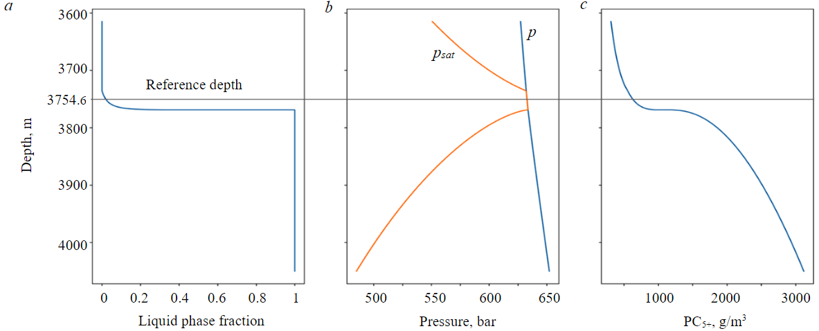
Fig.3. Results of the modified algorithm for composition 1 Calculated dependencies on depth for: a – molar fraction of the liquid phase; b – pressure p and saturation pressure psat, bar; c – PC5+, g/m3
From Fig.3, a it is evident that when moving upwards from the reference depth of 3754.6 m, the LHC fraction expectedly decreases, while it increases when moving downwards. The change in the LHC fraction from 0 to 1 occurs in the depth interval from 3736 to 3769 m. Within this interval, the reservoir pressure and the saturation (dew point) pressure are equal (Fig.3, b), indicating the two-phase state: the gas phase is saturated, and the liquid phase is present. Above and below this interval, the plots in Fig. 3, b do not match, indicating a transition to the single-phase region. Above the 3736 m level, the gas condensate mixture becomes undersaturated, with no LHC present. At the 3769 m level, the GOC is observed, and the LHC fraction reaches 100 %. When comparing Fig.2 and 3, it is apparent that considering LHC leads to the replacement of the supercritical gas-oil contact with the classical one and increase in PC5+ values (Fig.3, c), i.e., to higher condensate content in the reservoir gas.
Main parameters of the Composition 2 are close to the conditions of the main reservoir of the Orenburg OGCF. The reservoir fluid is modeled with a mixture of 23 components, including 15 pseudo-fractions (Table 2). The reference depth is h = 1250 m, pressure at the reference depth is р = 195 bar, temperature is Т = 29.34 °С, and the geothermal gradient is dT = 0.009 °С/m. At the reference point, the composition is saturated to the LHC molar fraction of 8% (L0 = 0.08).
The results of the modified algorithm are shown in Fig.4.
Table 2
Input data for composition 2
|
Components |
Molar fraction z, % |
Molar mass M, g/mol |
Critical temperature Tc, °С |
Critical pressure pc, bar |
Acentric factor ω |
Molar enthalpy Href, J |
Coefficients of cubic approximation for ideal gas heat capacity [38] |
|||
|
A |
B |
C |
D |
|||||||
|
N2 |
5.4704 |
28.013 |
–146.95 |
33.944 |
0.04 |
8330.789 |
31.1488 |
-0.0136 |
0.0 |
0.0 |
|
CO2 |
0.6595 |
44.01 |
31.55 |
73.866 |
0.225 |
19459.1011 |
19.7946 |
0.0734 |
–0.0001 |
0.0 |
|
H2S |
1.7432 |
34.076 |
100.45 |
89.369 |
0.1 |
12550.8657 |
31.9401 |
0.0014 |
0.0 |
0.0 |
|
C1 |
83.2209 |
16.043 |
–82.55 |
46.042 |
0.013 |
2.6425 |
19.2503 |
0.0521 |
0.0 |
0.0 |
|
C2 |
4.0362 |
30.07 |
32.28 |
48.839 |
0.0986 |
9761.1347 |
5.4092 |
0.1781 |
–0.0001 |
0.0 |
|
C3 |
1.7471 |
44.097 |
96.65 |
42.455 |
0.1524 |
19519.6224 |
–4.2244 |
0.3063 |
–0.0002 |
0.0 |
|
IC4 |
0.3152 |
58.124 |
134.95 |
36.477 |
0.1848 |
29278.1212 |
–1.39 |
0.3847 |
–0.0002 |
0.0 |
|
C4 |
0.6338 |
58.124 |
146.35 |
37.47 |
0.1956 |
29278.1212 |
9.487 |
0.3313 |
–0.0001 |
0.0 |
|
F1 |
0.9559 |
84.0 |
226.5 |
30.7 |
0.2706 |
34921.866 |
15.1105 |
0.4975 |
–0.0002 |
0.0 |
|
F2 |
0.436 |
94.0 |
264.5 |
30.92 |
0.324 |
39079.231 |
16.9094 |
0.5568 |
–0.0002 |
0.0 |
|
F3 |
0.2809 |
110.0 |
301.1 |
29.07 |
0.3566 |
45731.015 |
19.7876 |
0.6515 |
–0.0003 |
0.0 |
|
F4 |
0.1706 |
126.0 |
333.7 |
27.04 |
0.4078 |
52382.799 |
22.6658 |
0.7463 |
–0.0003 |
0.0 |
|
F5 |
0.1005 |
141.0 |
364.0 |
25.37 |
0.4764 |
58618.8465 |
25.3641 |
0.8351 |
–0.0003 |
0.0 |
|
F6 |
0.051 |
156.0 |
395.2 |
24.28 |
0.5427 |
64854.894 |
28.0624 |
0.924 |
–0.0004 |
0.0 |
|
F7 |
0.0378 |
173.0 |
424.8 |
23.03 |
0.6141 |
71922.4145 |
31.1205 |
1.0247 |
–0.0004 |
0.0 |
|
F8 |
0.0383 |
203.0 |
456.2 |
20.93 |
0.6437 |
84394.5095 |
36.5171 |
1.2024 |
–0.0005 |
0.0 |
|
F9 |
0.0292 |
220.0 |
487.7 |
20.58 |
0.7118 |
91462.03 |
39.5752 |
1.303 |
–0.0005 |
0.0 |
|
F10 |
0.025 |
273.0 |
514.4 |
17.3 |
0.728 |
113496.0645 |
49.1093 |
1.617 |
–0.0006 |
0.0 |
|
F11 |
0.0115 |
296.0 |
539.1 |
16.46 |
0.8339 |
123058.004 |
53.2467 |
1.7532 |
–0.0007 |
0.0 |
|
F12 |
0.0104 |
310.0 |
562.9 |
16.13 |
0.976 |
128878.315 |
55.7651 |
1.8361 |
–0.0007 |
0.0 |
|
F13 |
0.0074 |
356.0 |
588.9 |
14.64 |
1.0396 |
148002.194 |
64.0399 |
2.1086 |
–0.0008 |
0.0 |
|
F14 |
0.0019 |
372.0 |
605.0 |
14.29 |
1.1295 |
154653.978 |
66.9181 |
2.2033 |
–0.0009 |
0.0 |
|
F15 |
0.0173 |
565.0 |
668.8 |
10.58 |
1.1534 |
234891.1225 |
101.6364 |
3.3464 |
–0.0013 |
0.0 |
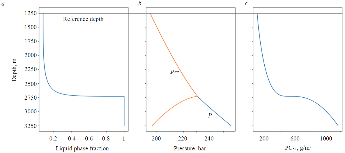
Fig.4. Results of the modified algorithm for composition 2 Calculated dependencies on depth for: a – molar fraction of the liquid phase; b – pressure p and saturation pressure psat, bar; c – PC5+, g/m3
Up to the depth of 2728 m, the saturation (dew point) pressure and the reservoir pressure are equal (Fig.4, b), indicating the presence of the saturated gas condensate mixture and LHC. The LHC fraction increases with depth, reaching 100 % at the 2728 m level, showing a classical GOC (Fig.4, a). Below the GOC, the reservoir pressure and saturation pressure no longer match (Fig.4, b), corresponding to the single-phase region with undersaturated oil – the oil rim. PC5+ values increase with depth quite uniformly in the gas condensate region and more intensively below the GOC (Fig.4, c), reflecting the specifics of increase in the content of heavy components.
Composition 3 models the conditions similar to the main reservoir of the Vuktyl OGCF. The fluid is represented by a mixture of 19 components (Table 3). The reference depth is h = 3025 m, pressure at the reference depth is р = 362.9 bar, temperature is Т = 61.4 °С, and the geothermal gradient is dT = 0.0175 °С/m. At the reference point, the composition is saturated to the LHC molar fraction of 14% (L0 = 0.14).
The results of the modified algorithm are presented in Fig.5.
Table 3
Input data for composition 3
|
Components |
Molar fraction z, % |
Molar mass M, g/mol |
Critical temperature Tc, °С |
Critical pressure pc, bar |
Acentric factor ω |
Molar enthalpy Href, J |
Coefficients of cubic approximation for ideal gas heat capacity [38] |
|||
|
A |
B |
C |
D |
|||||||
|
N2 |
4.8184 |
28.013 |
–146.8889 |
33.9912 |
0.045 |
8330.789 |
31.1488 |
–0.0136 |
0.0 |
0.0 |
|
CO2 |
0.0408 |
44.01 |
31.0556 |
73.8153 |
0.231 |
19459.1011 |
19.7946 |
0.0734 |
–0.0001 |
0.0 |
|
C1 |
72.8929 |
16.043 |
–82.5722 |
46.0432 |
0.0115 |
2.6425 |
19.2503 |
0.0521 |
0.0 |
0.0 |
|
C2 |
8.7255 |
30.07 |
32.2722 |
48.8011 |
0.0908 |
9761.1347 |
5.4092 |
0.1781 |
–0.0001 |
0.0 |
|
C3 |
3.5793 |
44.097 |
96.6722 |
42.4924 |
0.1454 |
19519.6224 |
–4.2244 |
0.3063 |
–0.0002 |
0.0 |
|
IC4 |
0.4663 |
58.124 |
134.9889 |
36.4802 |
0.1756 |
29278.1212 |
–1.39 |
0.3847 |
–0.0002 |
0.0 |
|
C4 |
0.8435 |
58.124 |
152.0278 |
37.9694 |
0.1928 |
29278.1212 |
9.487 |
0.3313 |
–0.0001 |
0.0 |
|
IC5 |
0.1743 |
72.151 |
187.2778 |
33.8119 |
0.2273 |
39036.6099 |
–9.5247 |
0.5066 |
–0.0003 |
0.0 |
|
C5 |
0.1409 |
72.151 |
196.5 |
33.6878 |
0.251 |
39036.6099 |
–3.6257 |
0.4873 |
–0.0003 |
0.0 |
|
C6P1 |
2.018 |
85.0188 |
250.9278 |
26.6887 |
0.1208 |
35345.4179 |
7.9027 |
0.5004 |
–0.0002 |
0.0 |
|
C6P2 |
3.138 |
110.457 |
318.9667 |
24.7149 |
0.2351 |
45921.0074 |
6.0966 |
0.6562 |
–0.0002 |
0.0 |
|
C6P3 |
1.815 |
157.953 |
398.0444 |
20.7256 |
0.3625 |
65666.8306 |
11.8058 |
0.9287 |
–0.0004 |
0.0 |
|
C6P4 |
0.5837 |
231.218 |
488.5167 |
16.8437 |
0.5589 |
96125.7653 |
22.824 |
1.3619 |
–0.0005 |
0.0 |
|
C6P5 |
0.299 |
338.184 |
586.3389 |
13.5525 |
0.7602 |
140595.426 |
42.4439 |
1.9968 |
–0.0008 |
0.0 |
|
C6P6 |
0.1931 |
500.0 |
679.6444 |
10.5933 |
1.0268 |
207868.25 |
75.7996 |
2.9481 |
–0.0011 |
0.0 |
|
C6P7 |
0.1216 |
598.0 |
674.6278 |
7.5153 |
1.3 |
248610.427 |
25.5721 |
3.407 |
–0.0014 |
0.0 |
|
C6P8 |
0.0778 |
794.1 |
737.6278 |
5.9157 |
1.481 |
330136.3547 |
33.1361 |
4.5271 |
–0.0018 |
0.0 |
|
C6P9 |
0.0475 |
1004.1 |
790.0722 |
4.8401 |
1.627 |
417441.0197 |
40.9978 |
5.7255 |
–0.0023 |
0.0 |
|
C6P10 |
0.0242 |
1284.2 |
845.0722 |
3.916 |
1.781 |
533888.7808 |
50.3553 |
7.3196 |
–0.0029 |
0.0 |
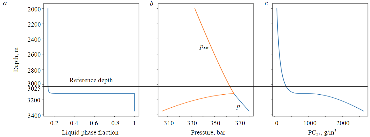
Fig.5. Results of the modified algorithm for composition 3 Calculated dependencies on depth for: a – molar fraction of the liquid phase; b – pressure p and saturation pressure psat, bar; c – PC5+, g/m3
For Composition 3, the change in the LHC fraction occurs up to the depth of 3120 m, where the LHC fraction reaches 100 %, and a classical GOC is observed (Fig.5, a). Below, the reservoir pressure and saturation pressure no longer match (Fig.5, b), corresponding to the single-phase undersaturated liquid state. The behavior of the PC5+ curve is similar to the Composition 2, but with more intensive increase below the GOC (Fig.5, c).
It is interesting to compare the results for Compositions 2 and 3 (Fig.6). Here the depth axis is relative, with the zero point set at the GOC level for each reservoir. The PC5+ plots for Compositions 2 and 3 are similar across almost the entire depth interval of the gas condensate region, excluding the interval near the GOC. Here, for Composition 3, the increase in the PC5+ is more gradual than for Composition 2 (Fig.6, b). However, the dependencies of the LHC fraction on depth differ significantly (Fig.6, a). For Composition 2, the LHC fraction smoothly increases throughout the depth interval down to the GOC. For Composition 3, a significant change in the LHC fraction is noted only when approaching the GOC level.
To analyze these differences, consider the depth variation of individual component fractions in the liquid phase obtained by the Negative Flash calculation. Plots of the component fractions from the top boundary of the calculation depths to the GOC are shown in Fig.7 for Compositions 2 and 3. It is noteworthy that the component С1 – methane – contributes most to the change in the LHC fraction (Fig.7, a, f). It can be observed that for Composition 2, the change in the methane fraction in the liquid phase is quite uniform throughout the entire calculated depth interval, while for Composition 3 significant changes begin near the GOC. A similar behavior is observed in the plot for the LHC fraction (Fig.7, e, j).
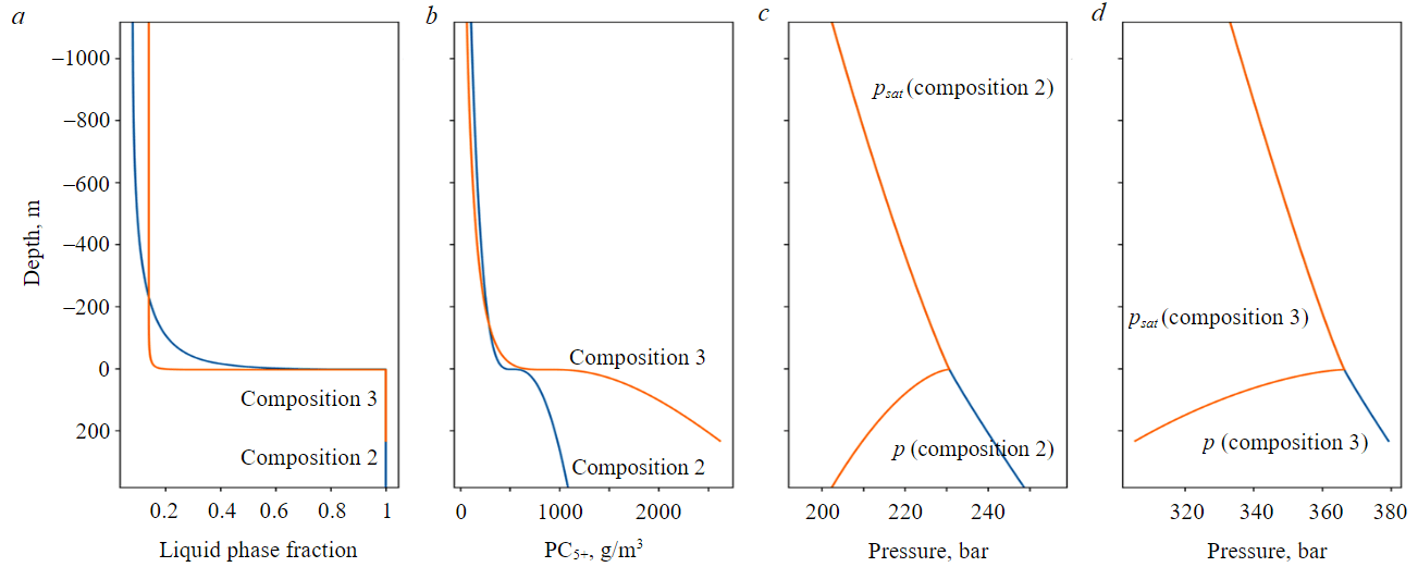
Fig.6. Comparison of the modified algorithm results for compositions 2 and 3 Calculated dependencies on depth for: a – molar fraction of the liquid phase, compositions 2 and 3; b – PC5+, g/m3, compositions 2 and 3; c – pressure p and saturation pressure psat, bar, composition 2; d – pressure p and saturation pressure psat, bar, composition 3
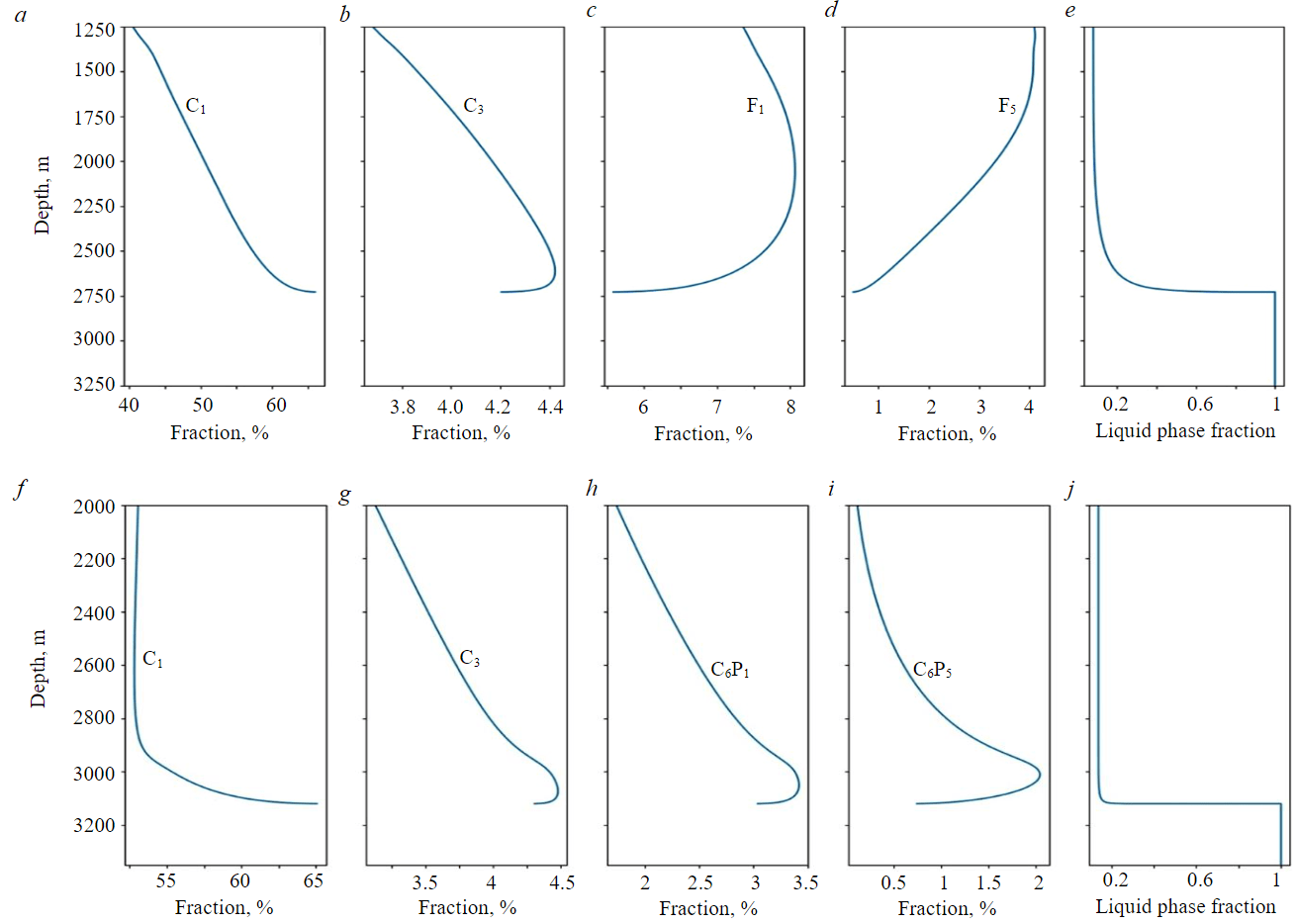
Fig.7. Plots of the molar component concentrations in the liquid phase for compositions 2 and 3 Calculated dependencies on depth for: a – molar fraction of methane, %; b – molar fraction of propane, %; c – molar fraction of group F1, %; d – molar fraction of group F5, %; e – molar fraction of the liquid phase (composition 2); f – molar fraction of methane, %; g – molar fraction of propane, %; h – molar fraction of group C6P1, %; i – molar fraction of group C6P5, %; j – molar fraction of the liquid phase (composition 3)
Thus, the character of the LHC fraction dependence on depth is determined by the swelling effect due to the dissolution of light components, particularly methane, which has the highest concentration in the liquid phase. It is important to note that the composition of the LHC in the gas condensate region of the reservoir changes with depth differently than in the oil region. The pressure and the fraction of intermediate components increase with depth in the gas phase, and consequently – in the liquid phase equilibrated with it. With an increased concentration of С3-С4 in the saturated liquid phase, the solubility of methane increases. This trend is opposite to the heaving of the liquid phase, characteristic for the undersaturated state below the GOC. It is worth noting that the noticeable sharp decrease in the content of intermediate and some heavy components near the GOC, as seen in Fig.7, is associated with the increase in methane content and normalization of concentrations.
Conclusion
The presence of a small fraction of scattered LHC in many gas condensate reservoirs necessitates changes in approaches to calculating the initial composition distribution with depth. In this case, classical methods of compositional grading are not applicable.
The modified algorithm for compositional grading discussed and implemented in this study makes it possible not to completely abandon the concept of quasi-equilibrium initial state of the hydrocarbon system, but to supplement it with necessary assumptions and calculation procedures for consistent consideration of the scattered LHC.
Calculation cases presented for different gas condensate mixtures, close by composition and conditions to real oil-gas-condensate reservoirs with significant hydrocarbon columns, demonstrate several characteristic features of the LHC impact on the compositional gradient: elevation and possible change of type for the fluid contact, as well as for the PC5+ dependency on depth. In regions with the LHC, the reservoir gas condensate fluid is saturated, and the saturation (dew point) pressure matches the reservoir pressure.
It is shown that the character of the LHC fraction change with depth can be different. Light components, particularly methane, contribute most, which is explained by the swelling effect of the saturated liquid phase. The change in the LHC composition with depth in the gas condensate part of the reservoir also shows significantly different trends than in the oil zone, where the liquid phase is undersaturated with light hydrocarbons.
The proposed approach to considering LHC, as well as the concept of quasi-equilibrium compositional gradient, allow calculating in a thermodynamically consistent way the initial state of oil-gas-condensate reservoirs with the presence of scattered LHC, estimating the GOC position and distribution of volumes in place for gas, liquid hydrocarbons, and individual components. The results of compositional grading considering LHC define the initial conditions when modeling field development and justifying technological solutions for efficient hydrocarbon recovery.
The presented method relies on assumptions of pseudo-equilibrium distribution of the gas phase with depth and local thermodynamic equilibrium between the gas condensate fluid and the scattered LHC. Their applicability to the conditions of specific oil-gas-condensate reservoirs requires further examination considering the formation specifics and accumulated actual data.
When analyzing the accuracy of the compositional gradient calculations, it is recommended to include a check of calculated concentrations of the C5+ group components at control points in depth. Typically, they are expected to satisfy the two-parameter gamma distribution [2]. For some reservoirs, it has been noted that the actual change in the concentrations of C5+ components with depth is predominantly linear [34].
Future refinements of the presented method could include accounting for capillary pressure and the gas-oil transition zone, for example, analogously to the work [39]. The current version of the method also predicts formation of a transition zone with the LHC saturation increasing to 100 % at the GOC (see Fig.3, a, 4, a, 5, a), but based on thermodynamics rather than on capillary effects.
References
- Brusilovskii A.I. Phase transitions in oil and gas field development. Moscow: Graal, 2002, p. 575 (in Russian).
- Whitson C.H., Brulé M.R. Phase behavior. Richardson: Society of Petroleum Engineers, 2000. Vol. 20, p. 240. DOI: 10.2118/9781555630874
- Novikov S., Weinheber P., Charupa M. et al. Tight Gas Achimov Formation Evaluation and Sampling with Wireline Logging Tools: Advanced Approaches and Technologies. SPE Russian Petroleum Technology Conference, 26-28 October 2015, Moscow, Russia. OnePetro, 2015. N SPE-176591-MS. DOI: 10.2118/176591-MS
- Gusev S., Garaev A., Zeybek M. et al. Reservoir Connectivity and Compartmentalization Detection with Down Hole Fluid Analysis Compositional Grading. SPE Russian Petroleum Technology Conference, 26-29 October 2020. OnePetro, 2020. N SPE-201895-MS. DOI: 10.2118/201895-MS
- Fundamentals of formation testing. Ed. by A.G.Zagurenko. Moscow, Izhevsk: Institut kompyuternykh issledovanii, 2012, p. 432 (in Russian).
- Aliev Z.S., Ismagilov R.N. Gas-hydrodynamic fundamentals of gas-condensate well testing. Moscow: Nedra, 2012, p. 214 (in Russian).
- Raupov I., Burkhanov R., Lutfullin A. et al. Experience in the Application of Hydrocarbon Optical Studies in Oil Field Development. Energies. 2022. Vol. 15. Iss. 10. N 3626. DOI: 10.3390/en15103626
- Asemani M., Rabbani A.R., Sarafdokht H. Implementation of an Integrated Geochemical Approach Using Polar and Nonpolar Components of Crude Oil for Reservoir-Continuity Assessment: Verification with Reservoir-Engineering Evidences. SPE Journal. 2021. Vol. 26. Iss. 5, p. 3237-3254. N SPE-205388-PA. DOI: 10.2118/205388-PA
- Kuklinsky A.Ya., Shtun S.Yu., Moroshkin A.N. Applying reservoir geochemistry methods to determine performance of each of jointly operated formations with different oil molecular composition. Geology, geophysics and development of oil and gas fields. 2021. N 1 (349), p. 39-43 (in Russian). DOI: 10.33285/2413-5011-2021-1(349)-39-43
- Dаntsova K.I., Iskaziyev K.O., Khafizov S.F. Geochemical characteristics of the organic matter of the Jurassic sediments of the southern regions of Western Siberia. Oil Industry. 2021. N 5, p. 50-53 (in Russian). DOI: 10.24887/0028-2448-2021-5-50-53
- Chen Q., Kristensen M., Johansen Y.B. et al. Analysis of Lateral Fluid Gradients from DFA Measurements and Simulation of Reservoir Fluid Mixing Processes over Geologic Time. Petrophysics. 2021. Vol. 62. Iss. 1, p. 16-30. N SPWLA-2021-v62n1a1. DOI: 10.30632/PJV62N1-2021a1
- Reitblat E.A., Zanochuev S.A., Goncharov I.V. et al. Study of gas composition and properties differentiation of Ach3–4 formation at the Novy Urengoy license area. Gas Industry Journal. 2021. N 12 (628), p. 46-52 (in Russian).
- Goncharov I.V., Veklich M.A., Oblasov N.V. et al. Nature of Hydrocarbon Fluids at the Fields in the North of Western Siberia: the Geochemical Aspect. Geochemistry International. 2023. Vol. 61. Iss. 2, p. 103-126. DOI: 10.1134/S0016702923020040
- Mukhametshin V.Sh., Khakimzyanov I.N. Features of grouping low-producing oil deposits in carbonate reservoirs for the rational use of resources within the Ural-Volga region. Journal of Mining Institute. 2021. Vol. 252, p. 896-907. DOI: 10.31897/PMI.2021.6.11
- Galkin S.V., Krivoshchekov S.N., Kozyrev N.D. et al. Accounting of geomechanical layer properties in multi-layer oil field development. Journal of Mining Institute. 2020. Vol. 244, p. 408-417. DOI: 10.31897/PMI.2020.4.3
- Ali Al-Amani Hj Azlan, Muda W.M.W., Mubaraki A.H et al. New Approach of Synergizing Advanced Well Test Deconvolution, Rate Transient Analysis and Dynamic Modeling in Evaluating Reservoir Compartmentalization Uncertainty at K Field in Sarawak Basin; A Case Study. SPE Middle East Oil and Gas Show and Conference, 18-21 March 2019, Manama, Bahrain. OnePetro, 2019. N SPE-195038-MS. DOI: 10.2118/195038-MS
- Pylev Ye.A., Churikov Yu.М., Polyakov Ye.Ye et al. Assessment of fault conductivity by well pressure interference tests: case of Chayanda oil-gas-condensate field. Vesti Gazovoy Nauki. 2021. Vol. 3 (48), p. 192-202 (in Russian).
- Plyusnin A.V., Gyokche M.I., Shavarov R.D., Nikulin E.V. Geodynamic and tectonic factors of the formation and destruction of carbonate Vendian-Cambrian hydrocarbon deposits in the south of the Nepa-Botuoba anteclise. Geosphere Research. 2023. N 1, p. 20-35 (in Russian).
- Pedersen K.S., Christensen P.L., Skaikh J.A. Phase behavior of petroleum reservoir fluids. Boca Raton: CRC Press, 2014, p. 465. DOI: 10.1201/b17887
- Høier L., Whitson C.H. Compositional Grading – Theory and Practice. SPE Reservoir Evaluation & Engineering. 2001. Vol. 4. Iss. 6, p. 525-535. N SPE-74714-PA. DOI: 10.2118/74714-PA
- Pedersen K.S., Hjermstad H.P. Modeling of Compositional Variation with Depth for Five North Sea Reservoirs. SPE Annual Technical Conference and Exhibition, 28-30 September 2015, Houston, TX, USA. OnePetro, 2015. N SPE-175085-MS. DOI: 10.2118/175085-MS
- Yazkov A.V., Gorobets V.E., Surkov E.V. et al. Complex Phase Behavior Study of a Near-Critical Gas Condensate Fluid in a Tight HPHT Reservoir. SPE Russian Petroleum Technology Conference, 26-29 October, 2020. OnePetro, 2020. N SPE-201997-MS. DOI: 10.2118/201997-MS
- Sajjad F.M., Chandra S., Ivan P. et al. The Effect of Compositional Gradient in Field Development. SPE/IATMI Asia Pacific Oil & Gas Conference and Exhibition, 12-14 October 2021. OnePetro, 2021. N SPE-205801-MS. DOI: 10.2118/205801-MS
- Gibbs J.W. The Collected Works of J. Willard Gibbs. Yale University Press, 1948. In 2 vol.
- Montel F., Gouel P.L. Prediction of Compositional Grading in a Reservoir Fluid Column. SPE Annual Technical Conference and Exhibition, 22-26 September 1985, Las Vegas, NV, USA. OnePetro, 1985. N SPE-14410-MS. DOI: 10.2118/14410-MS
- Haase R., Borgmann H.-W., Dücker K.-H., Lee W.-P. Thermodiffusion im kritischen Verdampfungsgebiet binärer Systeme. Zeitschrift für Naturforschung A. 1971. Vol. 26. Iss. 7, p. 1224-1227. DOI: 10.1515/zna-1971-0722
- Haase R. Thermodynamik der Irreversiblen Prozesse. Darmstadt: Dr. Dietrich Steinkopff Verlag, 1963, p. 554. DOI: 10.1007/978-3-642-88485-6
- Pedersen K.S., Lindeloff N. Simulations of Compositional Gradients in Hydrocarbon Reservoirs under the Influence of a Temperature Gradient. SPE Annual Technical Conference and Exhibition, 5-8 October 2003, Denver, Colorado. OnePetro, 2003. N SPE-84364-MS. DOI: 10.2118/84364-MS
- Pedersen K.S., Fredenslund A., Thomassen P. Properties of oils and natural gases. Houston: Gulf Publishing Company, 1989, p. 252.
- Popov S.B. Compositional grading by depth in gas and oil fields with temperature gradient. Keldysh Institute PREPRINTS. N 38, p. 32 (in Russian). DOI: 10.20948/prepr-2018-38
- Michelsen M.L. The isothermal flash problem. Part I. Stability. Fluid Phase Equilibria. 1982. Vol. 9. Iss. 1, p. 1-19. DOI: 10.1016/0378-3812(82)85001-2
- Popov S.B. Compositional grading with a depth in gas-oil reservoirs. Keldysh Institute PREPRINTS. N 61, p. 30 (in Russian). DOI: 10.20948/prepr-2017-61
- Whitson C.H., Belery P. Compositional Gradients in Petroleum Reservoirs. University of Tulsa Centennial Petroleum Engineering Symposium, 29-31 August 1994, Tulsa, OK, USA. OnePetro, 1994. N SPE-28000-MS. DOI: 10.2118/28000-MS
- Surnachev D.V., Skibitskaya N.A., Indrupskiy I.M., Bolshakov M.N. Assessment of the content and composition of liquid hydrocarbons of matrix oil in the gas-saturated part of productive deposits of oil and gas condensate fields: the case of the Vuktyl oil and gas condensate field. Actual Problems of Oil and Gas. 2022. Iss. 1 (36), p. 42-65 (in Russian). DOI: 10.29222/ipng.2078-5712.2022-36.art3
- Skibitskaya N., Bolshakov M., Burkhanova I. et al. Tight Oil in Oil-And-Gas Source Carbonate Deposits’ Gas Saturation Zones of Gas-Condensate and Oil-Gas Condensate Fields. SPE Russian Petroleum Technology Conference and Exhibition, 24-26 October 2016, Moscow, Russia. OnePetro, 2016. N SPE-182076-MS. DOI: 10.2118/182076-MS
- Kusochkova E.V., Indrupskiy I.M., Kuryakov V.N. Distribution of the Initial Fluid Composition in an Oil-Gas-Condensate Reservoir with Incomplete Gravity Segregation. IOP Conference Series: Earth and Environmental Science. 2021. Vol. 931. N 012012. DOI: 10.1088/1755-1315/931/1/012012
- Whitson C.H., Michelsen M.L. The negative flash. Fluid Phase Equilibria. 1989. Vol. 53, p. 51-71. DOI: 10.1016/0378-3812(89)80072-X
- Reid R.C., Prausnitz J.M., Poling B.E. The Properties of Gases and Liquids. McGraw-Hill, 1987, p. 741.
- Wheaton R.J. Treatment of Variations of Composition with Depth in Gas-Condensate Reservoirs. SPE Reservoir Engineering. 1991. Vol. 6. Iss. 2, p. 239-244. N SPE-18267-PA. DOI: 10.2118/18267-PA