Application of the support vector machine for processing the results of tin ores enrichment by the centrifugal concentration method
- 1 — Ph.D. Associate Professor Irkutsk National Research Technical University ▪ Orcid ▪ Elibrary ▪ Scopus ▪ ResearcherID
- 2 — Ph.D. Associate Professor Irkutsk National Research Technical University ▪ Orcid ▪ Scopus
- 3 — General Director OOO “Sibicon” ▪ Orcid ▪ Scopus
- 4 — Ph.D. Professor Irkutsk National Research Technical University ▪ Orcid ▪ Scopus
Abstract
The relevance of the research is due to the acquisition of new knowledge about the features of the applicability of the support vector machine, related to machine learning tools, for solving problems of mathematical modeling of mining and processing equipment. The purpose of the research is a statistical analysis of the results of semi-industrial tests of the Knelson CVD technology on tin raw materials using the support vector machine method and the development of mathematical models suitable for further optimization of the technological parameters of the equipment. The objects of research were the products obtained as a result of the operation of hydro-cyclones, as well as the technological parameters of the operation of centrifugal concentrators. The work uses classical methods of mathematical statistics, the least squares method for constructing a linear regression model, the support vector machine implemented on the basis of the Scikit-learn library, as well as the method of verifying the resulting models based on the ShuffleSplit library. A general description of the process of testing the Knelson concentrator with continuous controlled unloading in relation to the enrichment of tin ores is presented. The results obtained were processed using the support vector machine. Regression models are obtained in the form of polynomials of the second degree and in the form of radial basis functions. A significant non-linearity is shown in the dependence between the content of the valuable component in the tailings and the values of the technological parameters of the apparatus.
None
Introduction
Extraction and processing of mineral raw materials have always been key issues of national security of our country [1]. Almost all types of minerals have been discovered on the territory of the Russian Federation, and for some of them our country is among the world leaders: iron ores, nickel, copper, zinc, tungsten, etc. [2, 3]. The key metal that is used in various industries is tin. Due to its properties [4], tin is widely used in alloying, tinning, soldering, and, most importantly, in the electronic and microelectronic industries.
In the late 90s – early 2000s tin mining in the Russian Federation was almost completely stopped. In 2010 only 100 t of concentrate were produced, although the largest tin reserves in the world are concentrated on the territory of Russia – more than 2 million tons, of which more than three-quarters were calculated in categories A + B + C1. Leading positions in the tin-mining industry are traditionally occupied by China, which since the mid-1990s provides at least 30 % of the world’s metal production (about 900 deposits), and Indonesia (20 %). In the Russian Federation, there are currently more than 250 tin deposits on the state register (Fig.1).
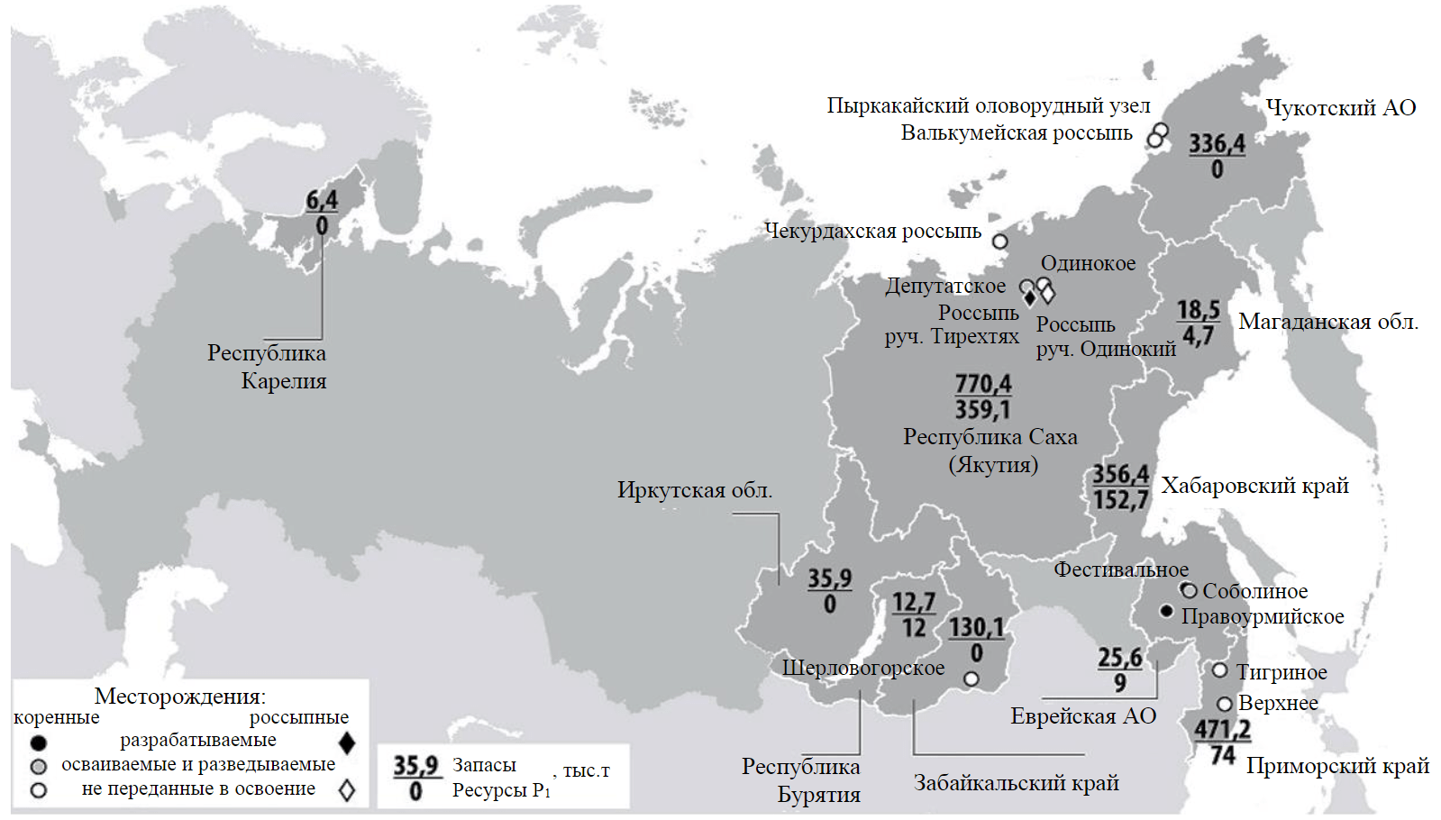
Fig.1. The state of the raw material base of tin in the Russian Federation
Materials and methods
The metal is mainly obtained from the processing of cassiterite, which, as a rule, is enriched using gravity methods and flotation enrichment. To achieve the highest reco-very efficiency at the stage of flotation enrichment, new reagent modes are used [5-7], new equipment is being designed, for example, the use of high-speed flotation in the grinding circuit deve-loped by Metso Outotec. The proposed technology makes it possible to minimize the regrinding of a valuable component, increase the productivity of extraction and reduce the watering of the enrichment circuit [8].
To extract large metal particles, gravitational enrichment is used, in particular, centrifugal concentration [9-11]. However, due to the peculiarities of the mineralogical composition [12] and the imperfection of the technologies used, a significant amount of a valuable component is lost with the tailings, which, with the right approach, can be extracted and processed.
There are various technologies for processing such materials, which are constantly updated [13, 14]. However, gravity and flotation enrichment remain the most common methods.
The use of centrifugal concentrators [15, 16] in gravitational methods for processing tin ores and products of their enrichment is an indicator of the modernity and efficiency of the raw material development scheme [17].
Manual tuning (technological parameters of centrifugal condensers, bowl rotation speed, the influence of the characteristics of the feedstock, valve operation, etc.) requires significant financial and time costs, therefore, when setting them up, mathematical modeling methods are most often used. The authors [18-20] attempted to develop a model for the operation of centrifugal concentrates based on classical regression approaches. However, the proposed solutions are not always suitable for obtaining a reliable model on enrichment tailings, since essentially non-linear dependencies when using classical methods do not allow taking into account the hidden relationships between the parameters of the concentrator. The purpose of this work is to describe the application of the support vector machine (related to machine learning methods) to the problem of constructing nonlinear models of the operation of a centrifugal concentrator based on polynomial radial basis functions of the kernel.
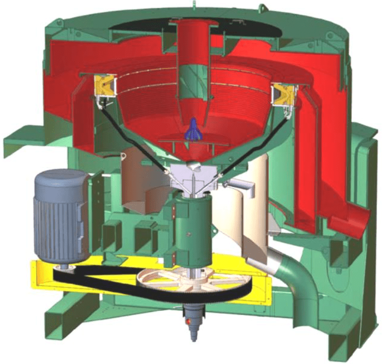
Fig.2. Concentrator Knelson KC-CVD64
The Knelson Continuous Variable Discharge (CVD) Concentrator is a centrifugal gravity separator designed to recover large masses of useful mineral that uses FLSmidth Knelson’s patented fluidization technology and pneumatic pinch valve system to ensure continuous concentrate output while fresh feed is added (Fig.2). CVD technology is mainly used for the extraction of base metals and industrial minerals (native copper, mercury, tantalite, cassiterite, chromite and scheelite [21-23], as well as precious metals [24, 25]).
The objects of research in this work were the products obtained as a result of the operation of hydrocyclones (hydraulic classifiers), as well as the technological parameters of the operation of centrifugal concentrators. The work used classical methods of mathematical statistics, the least squares method to build a linear regression model, the support vector method implemented on the basis of the Scikit-learn library, as well as the method of verification of the resulting models based on the ShuffleSplit library.
Methodology
Technological studies were carried out on three technological streams of the processing plant, namely, on the unloading of several spigots of a hydraulic classifier. After power was supplied to the semi-industrial plant, intermediate parameters were set, after which the preparatory stage was completed.
Unloading the first and second spigot of the hydraulic classifier
The combined product was fed by gravity to the plant. The solid content in this flow was about 40-50 %, the maximum particle size was 4 mm. In order to meet the requirements for the feed flow to the semi-commercial plant, follow-up water was added to the power supply pipeline and part of the flow was diverted through the plant bypass.
Stage 1. G-acceleration.
The tests were carried out at different rotor speeds – 60, 70, 80 and 90 G; productivity for solids was 1.73 t/h; average volume flow 1.44 m3/h; the content of tin in the diet is 1.24 %; the valve closing time was stopped for 8 s. On the basis of the set of tests carried out, the optimal rotor speed was established, which was 80 G, and the minimum value of the Sn content in the concentration tailings was fixed – 0.31 %. The maximum content of Sn in the tailings was established at a rate of 90 G – 0.44 %.
Stage 2. Fluidization water consumption.
Tests with different fluidized water flow setpoints during the enrichment cycle of the concentrator were carried out at a rotor speed of 80 G, a valve closing time of 12 s, a valve opening time of 0.32 s. The solid content in the food was 25 %, tin – 1.24 %. The flow rate of fluidization water varied from 25 to 45 l/min.
The best results were recorded at a water flow rate of 35 and 45 l/min – recovery was 75.75 and 88.45 %, respectively. However, the content in the concentrate of more than 2 % was achieved only at a flow rate of 45 l/min. For further tests, it was customary to use a fluidized water flow rate of 45 l/min.
Stage 3: Pinch valve opening frequency.
The next step was to establish the optimal value for the frequency of opening the pinch valves of the concentrator. Opening time 0.32 s; valve closing time – 18, 24, 32, 48, 64 s; the content of Sn in the diet is 1.24 %.
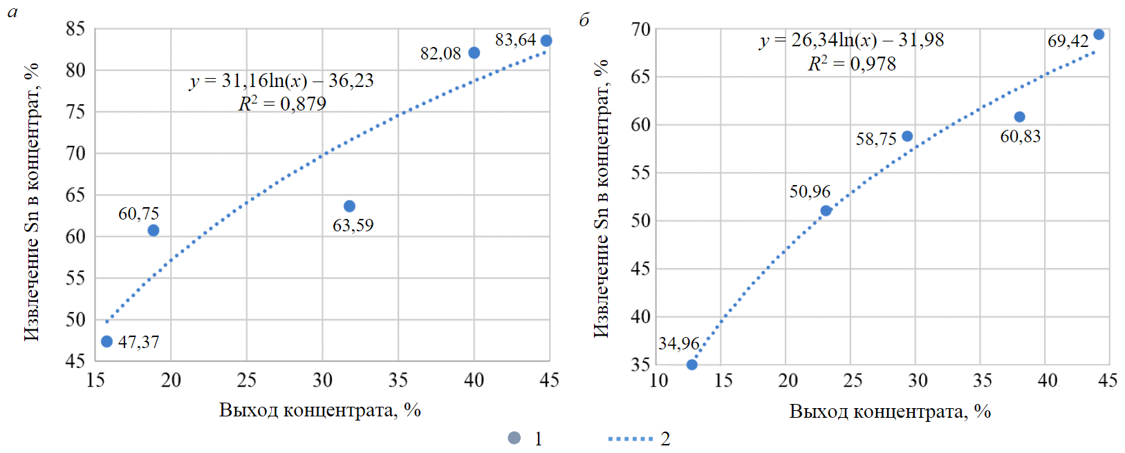
Fig.3. Dependences of extraction of Sn into concentrate on the output of concentrate during unloading of the first and second (а) and fourth (b) spigot hydraulic classifier 1 – dependence of Sn recovery on output; 2 – logarithmic dependence of Sn extraction into concentrate on the output
As a result of the experiment, it was found that with an increase in the valve closing time setting, the tin content in the concentrate increases linearly. Maximum content value in concentrate 3.23 % recorded at a valve closing time setpoint of 64 s. However, with increasing time, an increase in the concentration of the valuable component in the tailings is observed. Based on the data obtained, a graph of the dependence of the extraction of tin on the yield of the product was plotted (Fig.3, a). As a result of semi-industrial tests, the concentration coefficient varied from 1.7 to 3, the extraction of tin was 60-83 %.
Unloading the third spigot of the hydraulic classifier
On this process flow, a stable supply of material to the concentrator was ensured with an average solid content in the flow of 20-21 % with a particle size of –1+0 mm. Extraction did not fall below 80 % at a concentration of 1.51-1.76 and a tin content in the concentrate of 1.12-1.31 %. The best recovery rates in the concentrate were recorded at a rotor speed of 70 G and amounted to 87.84 %.
Based on the results of this test, the setpoint of the fluidized water flow rate was chosen to be 35 l/min. The extraction of tin into the concentrate was 88.93 %. The lowest recovery of the valuable component (80.55 %) was recorded at a flow rate of 40 l/min.
With an increase in the closing time of the pinch valves, the extraction of tin into the concentrate decreases from 82.6 to 42.35 %, while the concentrate yield decreases significantly – from 44 to 9 %.
It has been established that the technological performance of the concentrator is significantly affected by the size of the feed. For effective enrichment of the presented raw materials with a decrease in fineness, it is necessary to reduce the rotor speed and fluidization water consumption.
Unloading the fourth spigot of the hydraulic classifier
A similar set of studies was carried out on the unloading of the fourth spigot of the hydraulic classifier (Fig.3, b). On various technological streams a change in the concentration coefficient from 1.5 to 2.7 was established, while the recovery was fixed in the range of 34-70 %; the tin content in the concentrate varied from 2.78 to 3.65 g/t.
Discussion. As a result of the tests a data array of 33 experiments was obtained (see Table). The independent variables are the speed of rotation of the rotor х1, the flow rate of fluidization water х2, the time during which the valve is open х3 and the content of the valuable component in the feed х4. The content of the valuable component in the concentrate у1 and tailings у2 is taken as output variables.
The results of testing after applying the normalization procedure
|
Rotor speed х1 |
Fluid consumption water х2 |
Time х3 |
Input (Sn) х4, % |
Concentrate (Sn) у1, % |
Tails (Sn) у2, % |
|
–1.90502 |
–1.20829 |
–0.73582 |
0.449332 |
–0.85767 |
–0.10721 |
|
–0.64771 |
–1.20829 |
–0.73582 |
1.326049 |
–0.43093 |
–0.2532 |
|
0.609607 |
–1.20829 |
–0.73582 |
0.830513 |
–0.49494 |
–0.69117 |
|
1.866921 |
–1.20829 |
–0.73582 |
1.402285 |
–0.69764 |
0.257765 |
|
0.609607 |
–0.69045 |
–0.47726 |
–0.92292 |
–0.18556 |
0.841728 |
|
0.609607 |
–0.17261 |
–0.47726 |
1.859703 |
–0.50561 |
0.038779 |
|
0.609607 |
0.345225 |
–0.47726 |
1.211695 |
0.35852 |
–0.54518 |
|
0.609607 |
0.863064 |
–0.47726 |
–0.80857 |
0.145154 |
–0.39919 |
|
0.609607 |
1.380902 |
–0.47726 |
0.373096 |
1.094632 |
–0.2532 |
|
0.609607 |
1.380902 |
0.292669 |
1.135458 |
0.134485 |
0.33076 |
|
0.609607 |
1.380902 |
0.805954 |
2.317121 |
0.582554 |
1.133709 |
|
0.609607 |
1.380902 |
1.832523 |
–0.54174 |
1.382676 |
2.812602 |
|
0.609607 |
1.380902 |
2.859092 |
1.09734 |
1.553369 |
1.790667 |
|
0.609607 |
0.863064 |
0.804671 |
–0.84668 |
0.347851 |
1.644676 |
|
–1.90502 |
–0.69045 |
–0.47854 |
–0.84668 |
–0.49494 |
–1.05615 |
|
–0.64771 |
–0.69045 |
–0.47854 |
–0.69421 |
–0.54829 |
–1.34813 |
|
0.609607 |
–0.69045 |
–0.47854 |
–0.92292 |
–0.69764 |
–1.20214 |
|
1.866921 |
–0.69045 |
–0.47854 |
–1.07539 |
–0.58029 |
–1.20214 |
|
–0.64771 |
–1.20829 |
–0.47854 |
0.296859 |
–0.10022 |
–0.39919 |
|
–0.64771 |
–0.17261 |
–0.47854 |
0.525568 |
–0.14289 |
–0.10721 |
|
–0.64771 |
0.345225 |
–0.47854 |
0.525568 |
–0.12155 |
–0.69117 |
|
–0.64771 |
0.863064 |
–0.47854 |
–0.80857 |
–0.6123 |
–0.69117 |
|
–0.64771 |
1.380902 |
–0.47854 |
–0.73233 |
–0.6123 |
–0.98316 |
|
–0.64771 |
0.345225 |
–0.09358 |
0.030032 |
0.070475 |
–0.69117 |
|
–0.64771 |
0.345225 |
0.291386 |
–0.35115 |
–0.53762 |
–2.95403 |
|
–0.64771 |
0.345225 |
0.804671 |
–0.35115 |
0.742578 |
0.257765 |
|
–0.64771 |
0.345225 |
1.83124 |
–0.12244 |
2.438838 |
0.841728 |
|
–0.64771 |
0.345225 |
2.857809 |
0.220623 |
3.238961 |
1.863662 |
|
–1.90502 |
–1.20829 |
–0.47854 |
–0.80857 |
–0.85767 |
–0.39919 |
|
–0.64771 |
–1.20829 |
–0.47854 |
–1.15163 |
–1.02836 |
–0.2532 |
|
0.609607 |
–1.20829 |
–0.47854 |
–1.53281 |
–1.18838 |
–0.2532 |
|
1.866921 |
–1.20829 |
–0.47854 |
–1.45657 |
–1.07103 |
–0.83717 |
|
0.609607 |
1.380902 |
–0.73582 |
0.373096 |
–0.32425 |
0.549746 |
Processing of the obtained results to search for the most adequate model linking the input х1, х2, х3, х4 and the output у1, у2 process parameters, was carried out using the two most common metrics: the coefficient of determination R2 and the explained variance EV. The use of such a metric implies the division of the original data set into two parts – training and test sets:
where m is the number of vectors in the testing set; уi – true values of the parameter; – value calculated on the basis of the model; – the average value of the parameter in the calculation for the testing sample; D is the dispersion.
To eliminate the influence of the content of the samples (training and test) on the estimates of the models, cross-validation is used [26], when two subsets without repetitions are randomly selected from the initial sample k times. In this case the calculation of estimates is also carried out k times, and, thus, it is possible to obtain an estimate of the effectiveness of the model that is independent of the input data. Due to the small amount of initial data, we will divide the initial sample in the ratio of 80:20 for the training and testing parts, respectively, and take k equal to five.
When using such models, the most appropriate is the use of regression equations. First, consider a simple linear model for the variable y1 (determination coefficient R2 = 0.74 on the training set):
while the p-values of the regression coefficients calculated on the basis of t-statistics are equal to 0.69; 0.8; 0.14; 1.34·10–6; 0.15. Since all the coefficients, except for the coefficient at х3, are significantly greater than 0.05, then, despite the fact that there is a relationship between the variables under study, it is impossible to evaluate its quantitative characteristics using this equation.
Therefore, to search for a regression dependence between the variables under study, we propose to use other methods that allow us to establish not only a qualitative, but also a quantitative relationship between the factors [27]. So, along with the classical least squares method, one of the machine learning algorithms called the support vector machine (SVM) is used to solve regression analysis problems and construct complex nonlinear models. This approach is widely used to solve the classification problem; however, in the works [28-30], its applicability to solving regression problems is shown.
The support vector machine is used to map the original space R4∋x = (х1, х2, х3, х4)T into some hyperspace H. In this hyperspace, two parallel planes are built, the positions of which differ by the value of the parameter b. However, in order to build these hyperplanes, starting from some approximation, vectors are selected from the training set and added to the set of support SVs. After that, the objective function of the optimization problem being solved is determined – minimizing the deviation for all vectors that do not fall into the “gap” between the constructed hyperplanes, and the dual problem for this direct problem is also determined [30, 31].
The final regression equation looks like this:
where Di are the coefficients of the dual problem (with respect to the straight line, which consists in finding the coefficients of the hyperplane minimizing the penalty function); SV is the set of indices of support vectors; – the kernel used in the construction of hyperspace.
Consider the functions used in this algorithm as kernels. Thus, any function used as a kernel must satisfy the conditions of Mercer’s theorem [32], which requires non-negative definiteness and symmetry of the function in the space Rn. There are several standard functions used in software libraries that implement the support vector machine. Since it was found that linear regression did not bring a satisfactory result, two types of nonlinear kernels are used:
- polynomial kernel , where is the scalar product of vectors and ; p is the maximum degree of the polynomial;
- radial basis kernel , where is the distance metric between vectors; γ – parameter.
When using a polynomial kernel and the dimension of the feature space n = 4 with the opening of brackets, the kernel function appears in the following form:
where x1i … x4i are the coordinates of the i-th support vector.
Since we have only 33 observations, the use of the degree p > 2 will not be justified due to the fact that already at p = 3 the number of coefficients in the regression equation will be 33, so p = 2 is used for our problem. Then, when opening the brackets and inserting the kernel into expression (1) we get the regression equation for the polynomial kernel of the second degree
where α1… a14 are the coefficients obtained from the coordinates of the i-th support vector.
For the radial basis kernel, the function is written in the following form:
Substituting the regression equations into expression (1), we obtain:
where aij are the coefficients obtained from the coordinates of the i-th support vector.
The resulting regression function does not contain separate coefficients for the squares of the variables x1, x2, x3, x4, which makes it difficult to identify the impact on the output of each parameter separately; however, such a function can take into account a significant non-linear relationship between the inputs and outputs of the process.
For the software implementation of the support vector machine for the task of processing the test results of the CVD6 technology in the enrichment of tin ores, we will use the Scikit-learn library for the Python programming language. The ShuffleSplit method was used as a splitting strategy into training and testing samples, and the Numpy library was used to process data arrays.
Data obtained as a result of the program: with linear regression R2 = 0.614, EV = 0.722; with polynomial kernel SVM R2 = 0.693, EV = 0.781; with a radial-basic nucleus SVM R2 = 0.742, EV = 0.781. For the R2 and EV metrics the average results obtained after five runs are shown.
The use of both metrics of the SVM method showed the best results relative to simple linear regression, while for the R2 metric the radial basis kernel showed a slightly better result.
A feature of the support vector machine is the presence of the regularization hyperparameter C, the definition of which is individual both for each applied kernel function and for each problem being solved [30, 33, 34]. To find the best value of C we use a regular search over the segment C [ 0.0001; 10.0001] with a step of 0.0001 (Fig.4).
The final regression equations obtained with the best values of the hyperparameter C of the SVM method: for the polynomial kernel of the second degree the value corresponding to the maximum value of the EV metric, C = 0.0401, for the radial basis C = 2.943. Thus, the regression equation with a polynomial kernel is represented by the expression:
The value of the R2 metric calculated on the testing sample for this equation is 0.858, which is a high result.
After applying the support vector machine with a radial basis kernel to the problem being solved, the number of support vectors turned out to be 20 and, accordingly, equation (2) contains 20 terms, so we will present it in a general form:
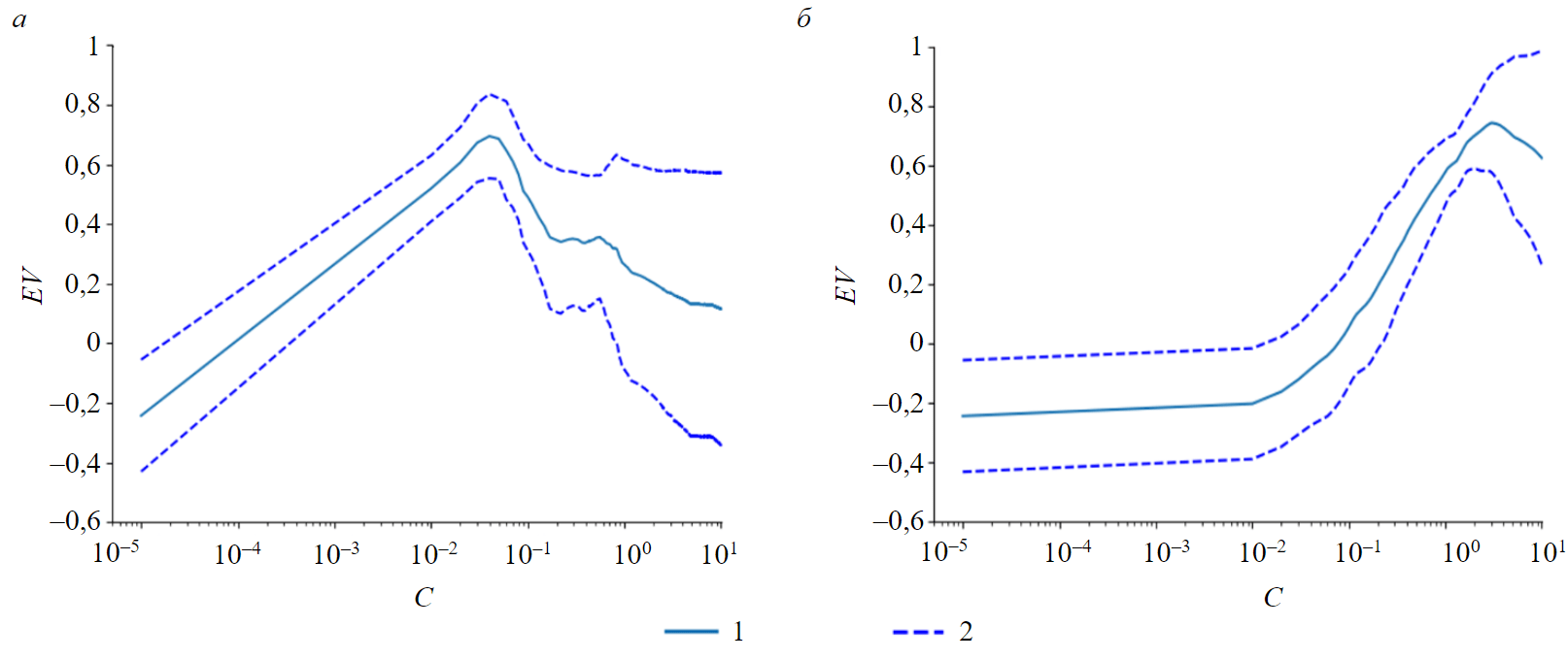
Fig.4. Graphs of fitting the hyperparameter C of the SVM method for the polynomial (a) and radial basic (b) kernels 1 – dependence of the metric on the value; 2 – standard deviation
Let us represent in the form of an array the values of the coefficients Bi = (–0.24; –0.13; –0.9; –2.19; –1.81; 2.45, 2.43; –1.17; 0.62; 1.39; –1.82; –0.53; –2.41; –5.96; 1.93; 3.47; –2.08; 3.36; 0.1; 2.81).
Since the total number of coefficients ai1; ai2; ai3; ai4 is equal to 80, they should not be given in the article. The value of the R2 metric calculated on the testing sample for this equation is 0.923, which corresponds to the high predictive ability of the model.
Let us present similar studies for tails. When using the polynomial kernel, the following regression equation was obtained:
The coefficient of determination R2, calculated on the testing sample, is 0.59, which is a low result.
For the radial basis kernel, the general form of the equation coincides with expression (4), and Bi has the following set of coefficients: Bi = (–0.33; 0.03; 0.54; 0.41; 0.64; 0.56; –0.75; –0.25; –0.49; 1.36; 0.19; 0.78; –1.51; –1.43; 0.14; –2.11; –2.23; –0.40; 0.05; 1.29; 1.11; –0.24; –0.58).
The value of the free coefficient b = 0.296, while R2 = 0.846.
The results obtained are in good agreement with the results obtained when working at processing plants with a different valuable component [18-20]. Therefore, models (3), (4) for the concentrate showed very good predictive ability on test samples (R2 > 0.85), while the use of a polynomial kernel is preferable, since it allows you to explore the resulting equation to find extreme points.
As a result, a stationary point M0 (–2.8; –3.47; – 1.83; 0.23) was found, the Hessian matrix corresponding to this point is sign-alternating. In this case the determinant of the largest minor is not equal to zero, which means that the found point M0 is a saddle point, i.e. the maximum values in the concentrate should be sought taking into account the restrictions imposed on the values of the variables х1, х2, х3, х4.
When using a polynomial kernel in the model for tails, unsatisfactory results are obtained, however, the model obtained on the basis of the radial basis kernel confirmed the thesis about the non-linear dependence of the content of the valuable component in the tails on the adjustable parameters.
Conclusion
It has been established that the support vector machine is applicable to the problem of processing the results of enrichment tests and shows quite interesting results. In particular, the tailings model obtained using the radial basis kernel convincingly indicates a significant non-linearity of the relationship between the content of the valuable component and the adjustable parameters, which will impose additional restrictions in the case of parametric optimization of the operation of the installation. Using the SVR support vector method with the radial basis kernel RBF we managed to obtain a model, which predictive ability has a fairly high result (R2 = 0.846).
The use of a polynomial kernel to find the relationship between the content of a valuable component in the concentrate and the adjustable parameters made it possible to obtain a high predictive ability R2 = 0.858 independent of the input data. At the same time, the use of a polynomial kernel made it possible to carry out a standard procedure for finding the extremum of a function of many variables with the resulting equation. The obtained values of the regression coefficients allow us to state that the most influential factor on the concentrate output is the time, during which the pinch valve is open, since the obtained coefficients of equation (3) have the highest absolute values of the terms, in which the variable х3 is present.
References
- Chanturiya V.A., Bocharov V.A. Modern state and basic ways of technology development for complex processing of non-ferrous mineral raw materials. Tsvetnye Metally. 2016. N 11, p. 11-18 (in Russian). DOI: 10.17580/tsm.2016.11.01
- Aleksandrova T.N., Orlova A.V., Taranov V.A. Enhancement of copper concentration efficiency in complex ore processing by the reagent regime variation. Journal of Mining Science. 2020. Vol. 56. Iss. 6, p. 982-989. DOI: 10.1134/S1062739120060101
- Fedotov P.K., Senchenko A.E., Fedotov K.V., Burdonov A.E. Studies of enrichment of sulfide and oxidized ores of gold deposits of the Aldan shield. Journal of Mining Institute. 2020. Vol. 242, p. 218-227. DOI: 10.31897/PMI.2020.2.218
- Angadi S.I., Sreenivas T., Ho-Seok Jeon et al. A review of cassiterite beneficiation fundamentals and plant practices. Minerals Engineering. 2015. Vol. 70, p. 178-200. DOI: 10.1016/j.mineng.2014.09.009
- Matveeva T.N., Chanturiya V.A., Getman V.V. et al. The Effect of Complexing Reagents on Flotation of Sulfide Minerals and Cassiterite from Tin-Sulfide Tailings. Mineral Processing and Extractive Metallurgy Review. 2022. Vol. 43. Iss. 3, p. 346-359. DOI: 10.1080/08827508.2020.1858080
- Leistner T., Embrechts M., Leißner T. A study of the reprocessing of fine and ultrafine cassiterite from gravity tailing residues by using various flotation techniques. Minerals Engineering. 2016. Vol. 96-97, p. 94-98. DOI: 10.1016/j.mineng.2016.06.020
- Matveeva T.N., Getman V.V., Karkeshkina A.Yu. Flotation extraction of tin from tailings of sulfide-tin ore dressing using thermomorphic polymer. Eurasian Mining. 2021. N 2, p. 46-49. DOI: 10.17580/em.2021.02.10
- Hassanzadeh A., Safari M., Duong H. Hoang et al. Technological assessments on recent developments in fine and coarse particle flotation systems. Minerals Engineering. 2022. Vol. 180. N 107509. DOI: 10.1016/j.mineng.2022.107509
- Angadi S.I., Eswaraiah C., Ho-Seok Jeon et al. Selection of Gravity Separators for the Beneficiation of the Uljin Tin Ore. Mineral Processing and Extractive Metallurgy Review. 2017. Vol. 38. Iss. 1, p. 54-61. DOI: 10.1080/08827508.2016.1262856
- Tong Yue, Haisheng Han, Yuehua Hu et al. Beneficiation and purification of tungsten and cassiterite minerals using Pb-BHA complexes flotation and centrifugal separation. Minerals. 2018. Vol. 8. Iss. 2. N 566. DOI: 10.3390/min8120566
- Zhang Jin-Lu, Ge Bao-Liang, Wang Xian-Qiang, Yang Chun-Gang. Study on Beneficiation of a Stanniferous Multi-metallic Sulphide Ore in Yunnan. The Chinese Journal of Process Engineering. 2015. Vol. 15. Iss. 6, p. 945-953. DOI: 10.12034/j.issn.1009-606X.215282
- Yusupov Т.S., Kondratyev S.А., Baksheeva I.I. Production-induced cassiterite-sulfide mineral for-mation structural-chemical and technological properties. Obogashchenie rud. 2016. N 5, p. 26-31 (in Russian). DOI: 10.17580/or.2016.05.05
- Yong Cheng Zhou, Xiong Tong, Xiao Wang et al. Beneficiation of Ultrafine Cassiterite from a Tin Tailings by Flotation. Advanced Materials Research. 2013. Vol. 616-618, p. 643-648. DOI: 10.4028/www.scientific.net/AMR.616-618.643
- Yongcheng Zhou, Xiong Tong, Shaoxian Song et al. Beneficiation of Cassiterite Fines from a Tin Tailing Slime by Froth Flotation. Separation Science and Technology. Vol. 49. Iss. 3, p. 458-463. DOI: 10.1080/01496395.2013.818036
- Murthy Y.R., Tripathy S.K. Process optimization of a chrome ore gravity concentration plant for sustainable development. Journal of the Southern African Institute of Mining and Metallurgy. 2021. Vol. 120. N 4, p. 261-268. DOI: 10.17159/2411-9717/990/2020
- Basnayaka L., Albijanic B., Subasinghe N. Performance evaluation of processing clay-containing ore in Knelson concentrator. Minerals Engineering. 2020. Vol. 152. N 106372. DOI: 10.1016/j.mineng.2020.106372
- Nayak A., Jena M.S., Mandre N.R. Application of Enhanced Gravity Separators for Fine Particle Processing: An Overview. Journal of Sustainable Metallurgy. 2021. Vol. 7. Iss. 2, p. 315-339. DOI: 10.1007/s40831-021-00343-5
- Pelikh V.V., Salov V.M., Burdonov A.E., Lukyanov N.D. Model of baddeleyite recovery from dump products of an apatite-baddeleyite processing plant using a CVD6 concentrator. Journal of Mining Institute. 2021. Vol. 248, p. 281-289. DOI: 10.31897/PMI.2021.2.12
- Pelikh V.V., Salov V.M., Burdonov A.E., Lukyanov N.D. Establishment of Technological Dependence of KC-CVD6 Concentrator Operation by Means of the Argument Group Accounting Method. Bulletin of the Tomsk Polytechnic University. Geo Assets Engineering. 2020. Vol. 331. N 2, p. 139-150 (in Russian). DOI: 10.18799/24131830/2020/2/2500
- Pelikh V.V., Salov V.M., Burdonov A.E., Lukyanov N.D. Application of Knelson CVD technology for beneficiation of gold-lead ore. Obogashchenie rud. 2019. N 1, p. 3-11 (in Russian). DOI: 10.17580/or.2019.01.01
- Sakuhuni G., Emre Altun N., Klein B. Modelling of continuous centrifugal gravity concentrators using a hybrid optimization approach based on gold metallurgical data. Minerals Engineering. 2022. Vol. 179. N 107425. DOI: 10.1016/j.mineng.2022.107425
- Koyzhanova A.K., Kenzhaliev B.K., Magomedov D.R., Abdyldaev N.N. Development of a combined processing technology for low-sulfide gold-bearing ores. Obogashchenie rud. 2021. N 2, p. 3-8 (in Russian). DOI: 10.17580/or.2021.02.01
- Majumder A.K., Barnwal J.P. Modeling of enhanced gravity concentrators – Present status. Mineral Processing and Extractive Metallurgy Review. 2006. Vol. 27. Iss. 1, p. 61-86. DOI: 10.1080/08827500500339307
- Fedotov P.K., Senchenko A.E., Fedotov K.V., Burdonov A.E. Integrated Technology for Processing Gold-Bearing Ore. Journal of the Institution of Engineers (India): Series D. 2021. Vol. 102. Iss. 2, p. 397-411. DOI: 10.1007/s40033-021-00291-0
- Jordens A., Sheridan R.S., Rowson N.A., Waters K.E. Processing a rare earth mineral deposit using gravity and magnetic separation. Minerals Engineering. 2014. Vol. 62, p. 9-18. DOI: 10.1016/j.mineng.2013.09.011
- Ojala M., Garriga G.C. Permutation Tests for Studying Classifier Performance. Journal of Machine Learning Research. 2010. Vol. 11, p. 1833-1863.
- Tie-Yan Liu. Learning to rank for Information Retrieval. Foundations and Trends in Information Retrieval. 2009. Vol. 3. N 3, p. 225-231. DOI: 10.1561/1500000016
- Vapnik V.N. An overview of statistical learning theory. IEEE Transactions on Neural Networks. 1999. Vol. 10. Iss. 5, p. 988-999. DOI: 10.1109/72.788640
- Ghanbari E., Shakery A. A Learning to rank framework based on cross-lingual loss function for cross-lingual information retrieval. Applied Intelligence. Vol. 52, p. 3156-3174. DOI: 10.1007/s10489-021-02592-z
- Sacks J., Welch W.J., Mitchell T.J., Wynn H.P. Design and analysis of computer experiments. Statistical Science. 1989. Vol. 4. Iss. 4, p. 409-423. DOI: 10.1214/ss/1177012413
- Smola A.J., Schölkopf B. A tutorial on support vector regression. Statistics and Computing. 2004. Vol. 14, p. 199-222. DOI: 10.1023/B:STCO.0000035301.49549.88
- Bartlett P., Shawe-Taylor J. Generalization Performance of Support Vector Machines and Other Pattern Classifiers. Advances in Kernel Methods. Cambridge: MIT Press, 1998, p. 43-54.
- Vapnik V., Izmailov R. V-matrix method of solving statistical inference problems. Journal of Machine Learning Research. 2015. Vol. 16, p. 1683-1730.
- Burdonov I.B., Vinarskii E.M., Yevtushenko N.V., Kossatchev A.S. Perfect Sets of Paths in the Full Graph of SDN Switches. Programming and Computer Software. 2021. Vol. 47. Iss. 7, p. 505-514. DOI: 10.1134/S0361768821070033