Increasing the efficiency of technological preparation for the production of the manufacture components equipment for the mineral resource complex
- 1 — Ph.D. Senior Lecturer Peter the Great Saint Petersburg Polytechnic University ▪ Orcid
- 2 — Ph.D. Director of the Higher School of Mechanical Engineering Peter the Great Saint Petersburg Polytechnic University ▪ Orcid
- 3 — Assistant Lecturer Peter the Great Saint Petersburg Polytechnic University ▪ Orcid ▪ Elibrary
- 4 — Assistant Lecturer Peter the Great St. Petersburg Polytechnic University ▪ Orcid

Abstract
An increase of components production for the equipment intended for oil and gas production is a key factor for analyzing existing technological processes and searching for new technological solutions to improve the efficiency of the production process and the quality of components. The article presents a simulation model designed to determine the rational technological processing parameters for the production of the “Centralizer shell” part. The basis for optimizing the working cycle of a production line is synchronization based on the principle of proportionality, which involves equalizing the duration of all technological operations with the rhythm of the production line. Synchronization of technological operations on the production line is carried out by choosing rational cutting parameters for each technological transition (cutting speed, feedrate, number of working passes). The “Centralizer shell” part is made of titanium alloy VT16, which has high strength, corrosion resistance and ductility. For the part under consideration, the permissible values of the cutting parameters were determined based on the calculation of the total processing error, as well as the frequency of replacement of the worn cutting tool. The simulation model described in the article made it possible to increase the efficiency of the production process due to the synchronization of technological operations and the search for rational technological parameters, as well as to improve the manufacturing quality of the “Centralizer shell” part by analyzing the processing error at various parameters of the technological process.
None
Introduction
In modern economic conditions, the mineral resource complex is one of the factors of sustainable development of the country. In Russia, the problems of oil and gas production are extremely important, since the industry largely fills the state budget and creates a large number of jobs [6, 9-11].
Currently, the main energy carriers are oil and gas, the processed products of which are used in almost all industries. Energy is the foundation of the Russian economy and the main driver of its development, in connection with which the issues of ensuring universal access to cheap, reliable, safe and environmentally friendly energy sources are a priority in the context of global sustainable development [1, 14, 15].
In the context of the imposition of sanctions and the prohibition of the import of oil and gas equipment, the issue of implementing the import substitution program arises. Many oil and gas companies are striving to embark on a digital transformation race where digital technologies are used to create new or transform traditional processes [16, 27, 35].
The potential to extract oil and gas from tight rock mass has increased rapidly over the past two decades. Drilling and stimulation technologies have improved, resulting in increased opportunities for oil and gas production from impermeable formations through precision directional drilling, massive multi-stage hydraulic fracturing and microseismic monitoring [20, 34].
For enterprises engaged in the production of equipment for the oil and gas industry, an increase in the production of components inevitably leads to the need to revise the existing technological processes in order to optimize them to increase the efficiency of the production process and maintain their competitiveness in the oil and gas equipment market in increased demand conditions.
Rising global energy consumption, growing demand for fossil fuels and increasing competition are driving the need to introduce advanced technologies into the production process [17, 18, 29]. In these conditions, increasing the efficiency of production processes directly depends on the quality of technological preparation of production, one of the main tasks of which is to determine the rational parameters of the technological process.
The most effective method for improving the quality of technological preparation of production is the simulation method [8, 13]. Control of technological processes based on simulation in mechanical engineering is one of the most promising areas of its development [3, 26].
Formulation of problem
One of the pressing problems in oil and gas production is the lowering of casing strings into wells, the quality of which depends on the preparedness of the wellbore and the intensity of the zenith angle change, the availability of a set of technical means to ensure high-quality lowering, as well as cementing the casing, which is carried out using a centralizer [7].
Currently, the most widespread are rigid centralizers due to the possibility of their use in wells with inclined and horizontal sections [5].
In connection with the increase in the volume of production of this type of product, it is necessary to develop a simulation model that allows determining rational parameters of the technological process, which reduce the labor intensity of manufacturing a product and increase its quality at the stage of technological preparation of production.
In the context of an increase in the production program for the manufacture of a “Centralizer shell” part, it seems rational to use a production line, the advantages of which include:
- increase in labor productivity due to a high level of automation, the use of specialized technological equipment and the constancy of traffic flows;
- reduction of the duration of the production cycle due to the high specialization of workplaces and the constant rhythm of their work;
- reducing the backlog of work in progress due to a significant reduction in the duration of the production cycle;
- improving the quality of products through detailed elaboration of the technological process, standardization and quality control of products;
- reducing the cost of manufactured products through the implementation of integrated solutions to optimize the production process.
One of the main tasks in the design of a production line is to reduce the time of breaks at the workplace by synchronizing technological operations. The method of synchronization of technological operations is the choice of the optimal combination of working strokes (processing patterns) and cutting parameters based on a preliminary analysis of the accuracy and productivity of processing [12, 19].
Currently, the problem of optimizing the operation of production lines is an urgent task in the framework of the technological preparation of production [22, 28]. The scientific literature contains a large number of simulation models, aimed at finding the optimal parameters of the production line, such as the duration of the production cycle, cutting parameters, the amount of interoperability breaks, etc. [21, 23, 31].
Issues of simulation and search for optimal parameters of assembly production lines are widely covered [25, 33, 36, 37]. A number of simulation models presented in the scientific literature [24, 30, 32], are based on logistic principles in modeling the production process.
The objective of the research is to develop a simulation model for a production line for the manufacture of a centralizer shell, which allows synchronizing the operation of its individual elements by determining rational cutting parameters based on the calculation and analysis of the total processing error.
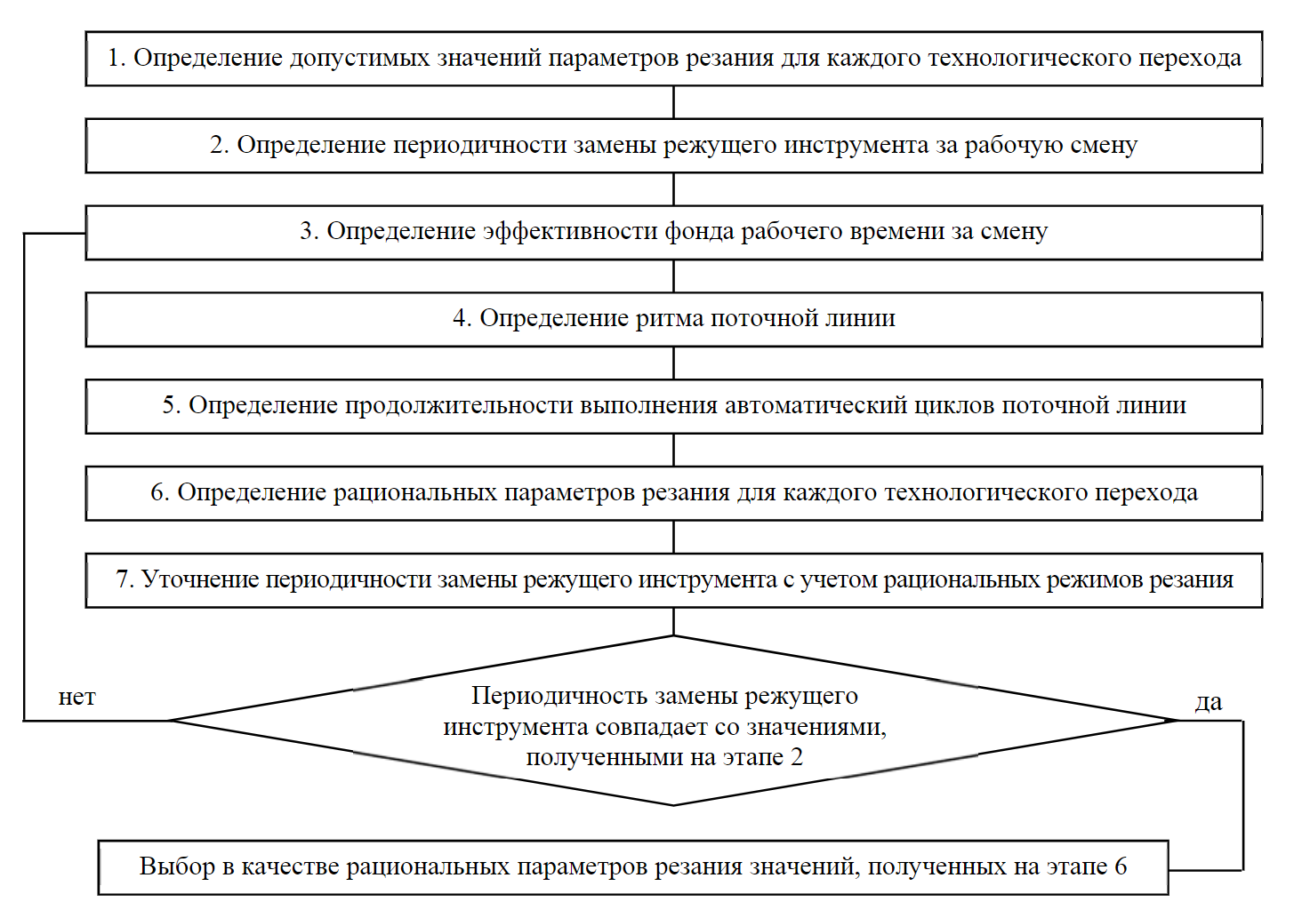
Fig.1. Simulation model diagram
Description of the simulation model
The centralizer shell is made of VT16 titanium alloy. The processing of parts made of titanium alloys is highly labor-intensive, therefore, the accuracy of their manufacture largely depends on the choice of optimal technological parameters [2].
The developed simulation model makes it possible to synchronize the operation of individual elements of the production line by coordinating the duration of interoperative breaks. The simulation model diagram consists of the following stages (Fig.1):
-
Determination of the permissible values of the cutting parameters (speed, depth of cut, feedrate) for each technological transition is based on the calculation of the total machining error, which should not exceed the size of tolerance field $IT(Δ_∑≤IT)$. In the case of processing in the structure of one instrumental transition of several surfaces with different tolerance fields, the determination of the permissible cutting parameters is carried out based on calculating the total processing error for the size, the tolerance field of which has a minimum value.
The calculation of the total processing error is based on the following components: the positioning error of the machine tool, the amount of wear of the cutting tool, thermal deformations of the cutting tool and part, elastic deformations of the technological system, random components of the processing error. For titanium alloys, the total processing error is determined by the formula [4]:
$$ y_i=2 \left[\Delta(i)+u(\tau,i)-\xi_\mathrm{cut}(i,\tau,u,t)- \xi_\mathrm d(\xi_\mathrm{cut})+\Delta_el(t,u)\right]+ \mathrmη_i,\qquad(1) $$where Δ(i) – otal positioning error, μm; u(i,τ) – cutting tool wear, μm; ξcut(i,τ,u,t) – thermal deformations of the cutting tool, μm; ξd(ξcut) – thermal deformation of the part, μm; Δel(t,u) – elastic deformations of the technological system, μm; – random components of the processing error, μm.
The calculation of the individual components of the total processing error is carried out according to the following formulas [7]:
$$ \Delta_i=K_1(i-1)+K_2;\qquad(2) $$$$ u(i,\mathrmτ)=K_3\mathrmτ+K_3(i-1)+K_4\Bigl(1-\mathrm{e}{(i-1+\mathrmτ)\over \mathrm{K}_5}\Bigl);\qquad(3) $$$$ \xi_\mathrm{cut}(i,\mathrmτ,u,t)=K_6t^{0,85}(1+K_7u)\Bigl(1-\mathrm{e}^{-{\mathrmτ\over \mathrm{K}_8}}\Bigl)+e^{{\mathrmτ_\mathrm{cool}\over 8}}\xi^{max}_{\mathrm{cut}(i-1)}e^{-{\mathrmτ\over K_8}};\qquad(4) $$$$ \xi_\mathrm{d}(\xi_\mathrm{cut})=K_9\xi_\mathrm{cut};\qquad(5) $$$$ \Delta_y(t,u)=K_{10}t(1+K_{11}u)(1-K_{12}\mathrmτ);\qquad(6) $$$$ \mathrmη_i=\pm3σ,\qquad(7) $$where i – part number in the batch; t – processing time of the i-th part; t – cutting depth; tcool – cooling time of the cutting tool before machining the i-th part; K1, ..., K2 – coefficients depending on the processing parameters (materials of the part and the cutting part of the tool, characteristics of technological equipment, etc.).
The output data of the first stage of modeling are the allowable values for each cutting parameter: $[V^\mathrm{add}_\mathrm{min};V^\mathrm{add}_\mathrm{max}]$, $[s^\mathrm{add}_\mathrm{min};Ss^\mathrm{add}_\mathrm{max}]$, $[t^\mathrm{add}_\mathrm{min};t^\mathrm{add}_\mathrm{max}]$, where $V^\mathrm{add}_\mathrm{min}$, $V^\mathrm{add}_\mathrm{max}$ – minimum and maximum allowable cutting speed; $s^\mathrm{add}_\mathrm{min}$, $s^\mathrm{add}_\mathrm{max}$ – minimum and maximum allowable feedrate values; $t^\mathrm{add}_\mathrm{min}$, $t^\mathrm{add}_\mathrm{max}$ – minimum and maximum allowable cutting depths.
-
The frequency of replacement of the cutting tool per work shift is determined based on the service life of the cutting tool, which depends on the cutting conditions. The task of this stage of modeling is a preliminary assessment of the frequency of replacement of each type of cutting tool used in the working cycle of the production line.
To estimate the tool life, the average values of the cutting parameters from the permissible intervals are used
$$ V^\mathrm{add}_\mathrm{av},s^\mathrm{add}_\mathrm{av},t^\mathrm{add}_\mathrm{av}\to T^\prime, \qquad(8) $$where $V^\mathrm{add}_\mathrm{av}$ – average cutting speed; $s^\mathrm{add}_\mathrm{av}$ – of feedrate;, $t^\mathrm{add}_\mathrm{av}$ – cutting depth from the permissible interval; $T^\prime$ – tool life period at average permissible values of cutting parameters.
The frequency of replacement of a worn-out cutting tool is determined by the formula:
$$ \mathrm{P_{ct}}={T_\mathrm{w.ct} \over {T^\prime}}={t_\mathrm{w.ct}N_\mathrm{shift} \over {T^\prime}},\qquad(9) $$where Tw.ct – operating time of the cutting tool per shift, min; tpart – operating time of the cutting tool for processing one part at average permissible cutting conditions, min; Nshift – number of processed parts per shift, pcs.
-
The effective fund of working time per shift for a production line can be determined by the formula:
$$ \mathrm{F_{shift}=D_{shift}}\cdot60-T_ \mathrm{change.ct}k, \qquad(10) $$where Dshift – working shift duration, h; $k=\sum\displaystyle^m_{i=1}(P_{ct})i$ – number of cutting tool units to be replaced per shift, pcs.; Pct – replacement frequency of the i-th cutting tool; m – the number of types of cutting tools required to machine a part; Тchange.ct – time required to replace one unit of the cutting tool, min.
-
Determination of the rhythm of the production line is made based on the effective fund of working time per shift and a given volume of parts production per shift
$$ r_\mathrm{pl}= {F_\mathrm{shift} \over N_\mathrm{shift}}. \qquad(11) $$ -
Determination of the duration of the execution of automatic cycles of the production line.
A production line cycle can be represented as a combination of two types of actions: auxiliary transitions and work cycles. Automatic cycles of processing parts on the machine are considered as working cycles. Ancillary actions include the delivery of blanks from the storage device to the machines and vice versa, moving the blanks between the machines, automatic control, installing and removing the blank, reinstalling the blank during the technological operation, etc.The duration of the working cycle of the production line is equal to the release rate and can be described by the following formula:
$$ R_{pl} = \sum\displaystyle_{i=1}^nAC_i+\sum\displaystyle_{j=i}^m(T_{вп})_j, \qquad(12) $$where ACi – duration of the i-th automatic cycle of the production line; (Tat)j – the duration of the j-th auxiliary transition of the production line; i – the number of automatic cycles; j – the number of auxiliary transitions in the working cycle of the production line.
The duration of each auxiliary transition is a constant value and is determined by the technical parameters of individual elements of the production line, the total duration of automatic cycles is determined by the formula:
$$ \sum\displaystyle_{i=1}^nAC_i = R_{pl}-\sum\displaystyle_{j=i}^m(T_\mathrm{at})_j. \qquad(13) $$ -
Determination of rational cutting parameters for each technological transition. According to the principle of proportionality, the duration of automatic cycles should be uniform, this helps to reduce the downtime of individual elements of the production line. The choice of rational cutting parameters from the permissible intervals is based on the condition $P_{pl} = \sum\displaystyle_{i=1}^nP_{i}=\mathrm{min}$ , where Ppl – the total amount of downtime on the production line; Pi – the amount of downtime by the elements of the production line.
The amount of downtime between the individual elements of the production line is determined by the formula:
$$ P_i=|R_{n-1}-R_n+T_\mathrm{tr}|,\qquad(14) $$where Rn-1 – production line duty cycle of (n – 1)-th element, s; – duty cycle of the production line n-th element duration; – time of blank transportation between (n – 1)-th and n-th elements of the production line, s.
The working cycle of the n-th machine includes the automatic machine cycle (blank cycle) Rn and auxiliary time (Tat)n:
$$ R_n=AC_n+(T_\mathrm{вп})_n; $$$$ {(T_{at})}_n=T_\mathrm{isnt.bl}+T_\mathrm{rem.bl}+T_\mathrm{add}, $$where ACn – automatic cycle time on the n-th machine; Tchange.ct – the time required to install the blank in the machine; Trem.bl – time required to remove the blank from the machine; Tadd –
the time required to complete additional auxiliary transitions provided by the production line work cycle.
The automatic cycle time of the machine depends on the number of technological transitions, the selected machining strategy and cutting parameters,
$$ AC_n=bT_\mathrm{change.st}+T_\mathrm{add}^{AC}+\sum\displaystyle_{i=1}^n{(T_\mathrm{wt}+T_\mathrm{a.trans})}_i, $$where Tchange.ct – – the cutting tool changing time, s; b – the number of tool transitions in the structure of the technological operation; Twt – time to complete work transitions included in the structure of the technological transition, s; Ta.trans – execution time of auxiliary transitions provided for in the structure of technological transition, s; m – number of instrumental transitions; $T_\mathrm{add}^{AC}$ – additional time required to implement the processing process, s.
The calculation of rational cutting parameters will be made based on the solution of a system of equations and inequalities:
$$ \begin{cases}P_\mathrm{pl}=\sum\displaystyle_{i=1}^nP_i=\mathrm{min};\\ \sum\displaystyle_{j=1}^mAC_j=R_\mathrm{pl}-\sum\displaystyle_{k=1}^m{(T_\mathrm{at})}_k;\\ {(V_\mathrm{min}^\mathrm{add})}_{1...r}≤V_{1...r}≤{(V_\mathrm{max}^\mathrm{add})}_{1...r};\\ {(s_\mathrm{min}^\mathrm{add})}_{1...r}≤s_{1...r}≤{(s_\mathrm{max}^\mathrm{add})}_{1...r};\\ {(t_\mathrm{min}^\mathrm{add})}_{1...r}≤t_{1...r}≤{(t_\mathrm{max}^\mathrm{add})}_{1...r}. \end{cases} $$ -
Clarification of the worn cutting tool replacement frequency is carried out taking into account the rational cutting conditions adopted based on the results of simulation carried out at stage 6. For each type of cutting tool, based on the adopted values of cutting conditions, the period of their durability is specified and the replacement frequency is calculated. Further, the total number of units of the cutting tool is determined, which must be replaced per shift, taking into account the accepted values of the cutting parameters (rational values):
$$ k^\prime=\sum\displaystyle_{i=1}^m({\mathrm P^\prime}_\mathrm{ct})_i,\qquad(15) $$where ${\mathrm P^\prime}_\mathrm{ct}$ – frequency of replacement of the i-th cutting tool, taking into account the adopted cutting conditions, min.
At this stage, two cases are considered. If k' = k, then the values obtained at stage 6 are taken as rational cutting parameters: Vrat=Vcalc; srat=scalc; trat=tcalc. If k' < k or k' > k, then there is a return to stage 3, and taking into account the value of the parameter k', repeated modeling of the production line operation and calculation of the parameters Vrat, srat, trat.
Determination of rational cutting parameters for the centralizer shell
The described simulation model was applied at the stage of technological preparation of production when designing a production line for the manufacture of a centralizer shell (Fig.2).
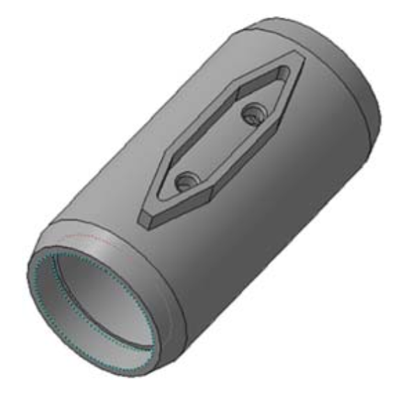
Fig.2. Centralizer shell
The developed technological process for the centralizer part contains two mechanical operations performed on CNC machines.
To implement the developed technological process, a production line was chosen, consisting of two machining centers, a storage device for blanks and finished products, as well as an automation system, which is designed to transport blanks between machines and a storage device.
At the first stage of modeling, the permissible intervals of cutting parameters were calculated. A Sandvik Coromant cutting tool was used to process the centralizer shell part. Based on the calculation of the total machining error, the permissible values for the cutting speed and feedrate were determined. The depth of cut for each technological transition was determined at the design stage of technological operations, therefore, when calculating the total processing error, this parameter was considered as a constant value “t = const”. For cutting speed and feedrate, the following permissible values of cutting parameters were obtained: external preliminary turning: V ∈ [50;69,2] m/min, s ∈ [0,1;0,27] mm/r; internal preliminary turning: V ∈ [50;68,2] m/min, s ∈ [0,1;0,26] mm/r; internal preliminary turning: V ∈ [50;78,9], s ∈ [0,08;0,29] mm/r; drilling: V ∈ [32;45,2] m/min, s ∈ [0,112;0,158] mm/r; milling: V ∈ [45;52,9] m/min, s ∈ [115;136,4] mm/r.
t the second stage, for each type of cutting tool, the frequency of its replacement was determined, taking into account the service life. The value of the tool life was calculated based on the average values of the cutting parameters belonging to the permissible interval. Depending on the processing method, the following values were obtained for the frequency of replacement of worn cutting tools during the shift: rough external turning – 4, rough boring – 3, fine boring – 2, drilling – 2, milling – 2. Time, required to replace one unit of a worn-out cutting tool was 2 min (120 s).
At the stage of simulation, the value of the effective fund of working time for a work shift was calculated. Taking into account the frequency of replacement of a worn-out cutting tool and accepted changeover time effective working hours per shift Fshift equal to 454 min.
The rhythm of the production line was determined taking into account the size of the effective fund of working time and the volume of production of parts per shift. According to the production plan, the number of manufactured parts per eight-hour shift is 75 pieces. Thus, the rhythm of the flow line rpl will be equal to 6.05 min (363.2 s).
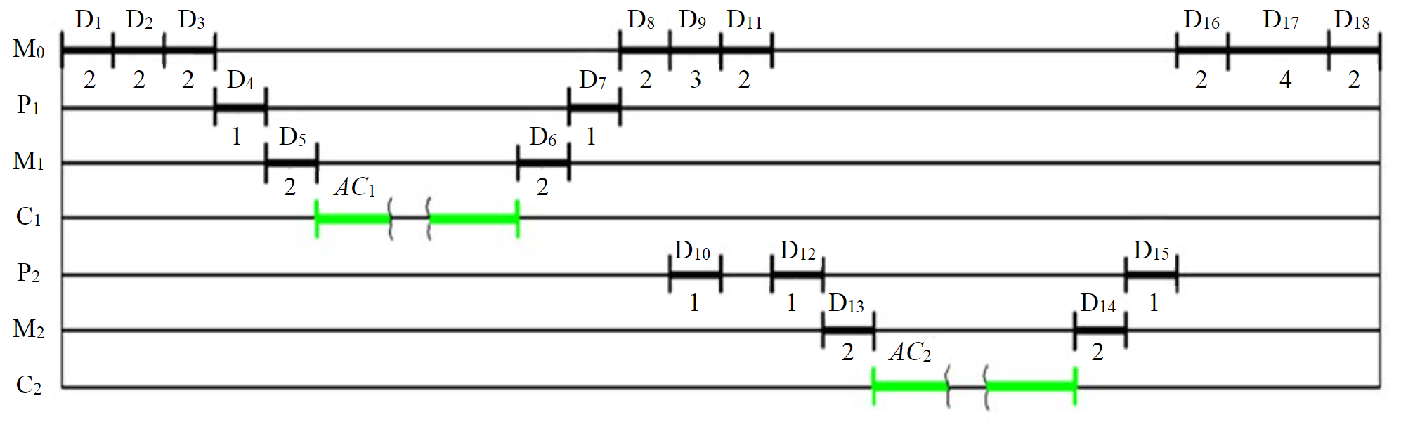
Fig.3. Cyclogram of the working cycle of the production line М0 – manipulator that moves blanks between the storage device and machines; С1 – machine 1; Р1 – pallet, with which the blanks are moved from the M0 manipulator to the working area of the machine С1; М1 – a manipulator that carries out the installation and removal of blanks in the working area of the machine С1; С2 – machine 2; Р2 – pallet, with which the blanks are moved from the M0 manipulator to the working area of the machine С2; М2 – a manipulator that carries out the installation and removal of blanks in the working area of the machine С2; B0 – a blank that has not been machined; B1 – blank after the first technological operation on the machine С1; B2 – blank after the second technological operation on the machine С2; D1 – taking the blank B0 from the storage; D2 – movement of the manipulator M0 from the storage device to the machine С1; D3 – installation of blank B0 on a pallet Р1; D4 – moving pallet P1 from manipulator M0 to the machine С1; D5 – installation of the blank B0 on the machine С1; D6 – removing the blank B1 from the machine C1 and placing it on the pallet Р1; D7 – moving pallet P1 from machine C1 to manipulator М0; D8 – taking the blank B1 by the manipulator М0; D9 – movement of the manipulator M0 from the C1 machine to the machine С2; D10 – moving pallet P2 from the C2 machine to the manipulator М0; D11 – installation of blank B1 on a pallet Р2; D12 – moving pallet P2 from the manipulator M0 to the machine С2; D13 – installation of blank B1 on the machine С2; D14 – removal of the blank B2 from the machine С2; D15 – moving pallet P2 from the machine C2 to the manipulator М0; D16 – taking blank B2 off the pallet Р2; D17 – movement of the manipulator M0 from the C2 machine to the storage; D18 – installation of blank B2 into the storage; AC1 – automatic cycle on the first machine; AC2 – automatic cycle on the second machine
According to the cyclogram (Fig.3), the value of the auxiliary time of the working cycle of the production line will be $\sum\displaystyle_{j=1}^m{(T_\mathrm{at})}_j= 34\quad \mathrm c,$, then the total execution time of automatic cycles will be equal to:
utomatic cycle 1 (AC1) has the following parameters: number of instrumental transitions b = 4; additional time required to implement the processing route, $T^{AC}_\mathrm{add}= 0 \quad \mathrm c;$ total time of auxiliary transitions $\sum\displaystyle_{i=1}^n(T_\mathrm{a.trans})_i=6,21 \quad \mathrm c.$
Automatic cycle 2 (AC2) has the following parameters: number of instrumental transitions b = 5; additional time required to implement the processing route, $T^{AC}_\mathrm{add}= 0 \quad \mathrm c;$ otal time of auxiliary transitions $\sum\displaystyle_{i=1}^n(T_\mathrm{a.trans})_i=3,29 \quad \mathrm c.$
For both automatic cycles, the cutter change time is 2 s. Thus, the equations for describing the duration of automatic cycles will be as follows:
where V1,...,V9 – cutting speeds for tool transitions cutting speeds for tool transitions 1, …, 9; s1,...,s9 – feedrades for tool transitions 1, …, 9.
The duration of the working cycle on the first machine at (Ta.trans)1=14 s can be described by the following equation:
The duration of the working cycle on the second machine at (Ta.trans)2 = 10 can be described by the following equation:
Transport time of the blank between the machines Ttrans = 3 с.
According to formula (14), the amount of downtime for the considered production line is determined by the formula:
For efficient operation of the production line, it is necessary that the amount of downtime is minimal
Determination of rational cutting parameters for the considered production line will be made based on the following system of equations and inequalities:
Because of modeling the production line operation based on the described equation system, the values of the cutting parameters were obtained, which can be taken as rational.
For the first automatic cycle, the following values of four technological transitions were obtained: V1 = 58,2, s1 = 0,19; V2 = 61,4, s2 = 0,21; V3 = 37,4, s3 = 0,64; V4 = 52,9 m/min, s4 = 0,213 mm/r.
For the second automatic cycle, the following values of five technological transitions were obtained: V5 = 61,9, s5 = 0,18; V6 = 47,3, s6 = 123,4; V7 = 49,4, s7 = 125,3; V8 = 37,1, s8 = 0,142; V9 = 48,1 m/min, s9 = 1 mm/r.
According to the results of calculations, the frequency of tool replacement based on the obtained values of the cutting parameters remained the same (k = k'), as a result, the presented values can be taken as rational cutting parameters for machining the centralizer shell.
Conclusion
The use of the developed simulation model at the stage of technological preparation of production for manufacturing the centralizer shell made it possible to increase the efficiency of the production process by reducing the duration of interoperation breaks, to improve the quality of products by calculating and analyzing the total processing error, to determine rational cutting parameters.
References
- Litvinenko V.S., Tsvetkov P.S., Dvoynikov M.V., Buslaev G.V. Barriers to implementation of hydrogen initiatives in the context of global energy sustainable development. Journal of Mining Institute. 2020. Vol. 244, p. 428-438. DOI: 10.31897/PMI.2020.4.5
- Maksarov V.V., Kosheleva E.V., Vazhenin A.Yu. Technological support of the quality of precision surfaces of the part of the type of “revolution bodies” from titanium alloys. Metalloobrabotka. 2018. N 4 (106), p. 52-59 (in Russian).
- Maksarov V.V., Rakhmankulov R.R. Technological support of the parameters of accuracy and roughness of beds based on the improvement of face milling on CNC machines. Vestnik Rybinskoi gosudarstvennoi aviatsionnoi tekhnicheskoi akademii im. P.A.Soloveva. 2017. N 1 (40), p. 268-276 (in Russian).
- Kozar I.I., Kolodyazhniy D.Yu., Radkevich M.M., Tsimko T.A. A Mathematical model of error for intractable alloy turning. Nauchno-tekhnicheskie vedomosti Sankt-Peterburgskogo gosudarstvennogo universiteta. 2014. N 2 (195), p. 194-201 (in Russian).
- Kozhevnikov E.V., Nikolaev N.I., Rozentsvet A.V., Lyrchikov A.A. Centering equipment for casing columns in sidetrack cementing. Vestnik Permskogo natsionalnogo issledovatelskogo politekhnicheskogo universiteta. Geologiya. Neftegazovoe i gornoe delo. 2015. N 16. P. 54-60. DOI: 10.15593/2224-9923/2015.16.6 (in Russian).
- Poddubny Yu.A., Poddubny A.Yu. Methods to increase oil return in the world: today and possible tomorrow. Burenie i neft. 2020. N 12, p. 43-49 (in Russian).
- Khuzina L.B., Fazlyeva R.I., Gabzalilova A.Kh. Improving the quality of well casing. Delovoi zhurnal Neftegaz.ru. 2018. N 1 (73), p. 88-91 (in Russian).
- Lyubomudrov S.A., Khrustaleva I.N., Tolstoles A.A., Maslakov A.P. Improving the efficiency of technological preparation of single and small batch production based on simulation modeling. Journal of Mining Institute. 2019. Vol. 240, p. 669-677. DOI: 10.31897/PMI.2019.6.669
- Razmanova S.V., Andrukhova O.V. Oilfield service companies as part of economy digitalization: assessment of the pros-pects for innovative development. Journal of Mining Institute. 2020. Vol. 244, p. 482-492. DOI: 10.31897/PMI.2020.4.11
- Kolevatov A.A., Afanasev S.V., Zakenov S.T. et al. Status and prospects for increasing oil refund formations in Russia (Part 1). Burenie i neft. 2020. N 12, p. 3-19 (in Russian).
- Sharf I.V., Afanaskin I.V., Volpin S.G. et al. Status and prospects for increasing oil refund formations in Russia (Part 2). Burenie i neft. 2021. N 1, p. 3-22 (in Russian).
- Maksarov V.V., Keksin A.I., Filipenko I.A., Brigadnov I.A. Technological features of magnetic abrasive machining in digital technologies. Metalloobrabotka. 2019. N 4 (112), p. 3-10 (in Russian).
- Khrustaleva I.N., Lyubomudrow S.A., Romanov P.I. Simulation model of technological preparation of production of the machining shop. Nauchno-tekhnicheskie vedomosti SPbPU. Estestvennye i inzhenernye nauki. 2017. Vol. 23. N 2, p. 215-222. DOI: 10.18721/JEST.230219 (in Russian).
- Chernysheva E. Modern aspects of development of oil refining in Russia. Burenie i neft. 2015. N 5, p. 4-8 (in Russian).
- Ali J.A., Kalhury A.M., Sabir A.N. et al. A state-of-the-art review of the application of nanotechnology in the oil and gas industry with a focus on drilling engineering. Journal of Petroleum Science and Engineering. 2020. Vol. 191. N 107118. DOI: 10.1016/j.petrol.2020.107118
- Abdulrahman I., Máša V., Teng S.Y. Process intensification in the oil and gas industry: A technological framework. Chemical Engineering and Processing – Process Intensification. 2021. Vol. 159. N 108208. DOI: 10.1016/j.cep.2020.108208
- Khalil M., Jan B.M., Tong C.W., Berawi M.A. Advanced nanomaterials in oil and gas industry: Design, application and challenges. Applied Energy. 2017. Vol. 191, p. 287-310. DOI: 10.1016/j.apenergy.2017.01.074
- Asl M.G., Canarella G., Miller S.M. Dynamic asymmetric optimal portfolio allocation between energy stocks and energy commodities: Evidence from clean energy and oil and gas companies. Resources Policy. 2021. Vol. 71. N 101982. DOI: 10.1016/j.resourpol.2020.101982
- Khrustaleva I.N., Lyubomudrov S.A., Chernykh L.G. et al. Automating production engineering for custom and small-batch production on the basis of simulation modeling. International Conference on Innovations, Physical Studies and Digitalization in Mining Engineering (IPDME) 2020, 23-24 April, 2020, St. Petersburg, Russian Federation. Journal of Physics: Conference Series, 2021. Vol. 1753. N 012047. DOI: 10.1088/1742-6596/1753/1/012047
- Boak J., Kleinberg R. Shale Gas, Tight Oil, Shale Oil and Hydraulic Fracturing t. Future Energy (Third Edition). Improved, Sustainable and Clean Options for our Plane. Elsevier, 2020, p. 67-95. DOI: 10.1016/B978-0-08-102886-5.00004-9
- Bulenkov Y. Structure of a products flow in multi-nomenclature rotary lines with regard to tool change times. IOP Conference Series: Materials Science and Engineering. 2018. Vol. 400. Iss. 2. N 022014. DOI: 10.1088/1757-899X/400/2/022014
- Ding S., Yang D., Han Z. Flow line machining of turbine blades. Proceedings. International Conference on Intelligent Mechatronics and Automation. 2004, p. 140-145. DOI: 10.1109/ICIMA.2004.1384177
- Gwiazda A., Sękala A., Banaś W. Modeling of a production system using the multi-agent approach. ModTech International Conference – Modern Technologies in Industrial Engineering V, 14-17 June, 2017, Sibiu, Romania. IOP Conference Series: Materials Science and Engineering, 2017. Vol. 227. N 012052. DOI: 10.1088/1757-899X/227/1/012052
- Humbeck P., Mangold S., Bauernhansl T. Future Scenarios of Value Creation in Mechanical Engineering – Derivation of Recommendations for Action. 53rd CIRP Conference on Manufacturing Systems, 1-3 July, 2020, Chicago, USA. Procedia CIRP, 2020. Vol. 93, p. 844-849. DOI: 10.1016/j.procir.2020.03.093
- Ma K., Chen Y., Sun Y. Mechanical System Design and Simulation Research of a Demonstration Assembly Line. 2019 2nd International Conference on Mechanical Manufacturing and Industrial Engineering, 14-16 December, 2019, Beijing, China. IOP Conference Series: Materials Science and Engineering, 2020. Vol. 784. N 012026. DOI: 10.1088/1757-899X/784/1/012026
- Muthanna J., Razali N.M. Simulation of Assembly Line Balancing in Automotive Component Manufacturing. 2nd International Manufacturing Engineering Conference and 3rd Asia-Pacific Conference on Manufacturing Systems (IMEC-APCOMS 2015), 12-14 November, 2015, Kuala Lumpur, Malaysia. IOP Conference Series: Materials Science and Engineering, 2016. Vol. 114. N 012049. DOI: 10.1088/1757-899X/114/1/012049
- Lu H., Guo L., Azimi M., Huang K. Oil and Gas 4.0 era: A systematic review and outlook. Computers in Industry. 2019. Vol. 111, p. 68-90. DOI: 10.1016/j.compind.2019.06.007
- Blaga F.S., Stănășel I., Pop A. et al. Performance evaluation of the support bush manufacturing line by modeling and simulation. Annual Session of Scientific Papers “IMT ORADEA 2019”, 30-31 May, 2019, Oradea, Felix SPA, Romania. IOP Conference Series: Materials Science and Engineering, 2019. Vol. 568. N 012030. DOI: 10.1088/1757-899X/568/1/012030
- Lei Q., Xu Y., Yang Z. et al.Progress and development directions of stimulation techniques for ultra-deep oil and gas reservoirs. Petroleum Exploration and Development. 2021. Vol. 48. Iss. 1, p. 221-231. DOI: 10.1016/S1876-3804(21)60018-6
- Pschybilla T., Homann A. Evaluation of end-to-end process and information flow analyses through digital transformation in mechanical engineering. 53rd CIRP Conference on Manufacturing Systems, 1-3 July, 2020, Chicago, USA. Procedia CIRP, 2020. Vol. 93, p. 298-303. DOI: 10.1016/j.procir.2020.04.070
- Weikang Fang, Zailin Guan, Dan Luo et al. Research on Automatic Flow-shop Planning Problem Based on Data Driven Modelling Simulation and Optimization. International Conference on Intelligent Manufacturing and Intelligent Materials (2IM 2019), 9-11 May, 2019, Sanya, China. IOP Conference Series: Materials Science and Engineering, 2019. Vol. 565. N 012005. DOI: 10.1088/1757-899X/565/1/012005
- Wentao L., Yan R., Jianfu Z., Linjiang D. Research on Simulation Decision of Logistics in Flexible Factory. 3rd International Conference on Data Mining, Communications and Information Technology (DMCIT 2019), 24-26 May, 2019, Beijing, China. IOP Conference Series: Journal of Physics: Conference Series, 2019. Vol. 1284. N 012015. DOI: 10.1088/1742-6596/1284/1/012015
- Revina I.V., Trifonova E.N. Simulation modeling of the assembly process. XIII International Scientific and Technical Conference “Applied Mechanics and Systems Dynamics”, 5-7 November, 2019, Omsk, Russian Federation. Journal of Physics: Conference Series, 2020. Vol. 1441. N 012110. DOI: 10.1088/1742-6596/1441/1/012110
- Senderov S.M., Vorobev S.V. Approaches to the identification of critical facilities and critical combinations of facilities in the gas industry in terms of its operability. Reliability Engineering & System Safety. 2020. Vol. 203. N 107046. DOI: 10.1016/j.ress.2020.107046
- Castiñeira D., Darabi H., Zhai X., Benhallam W. Smart reservoir management in the oil and gas industry. Smart Manufacturing. Elsevier, 2020, p. 107-141. DOI: 10.1016/B978-0-12-820028-5.00004-7
- Yasir A.S.H.M., Mohamed N.M.Z.N. Assembly Line Efficiency Improvement by Using WITNESS Simulation Software. The 4th Asia Pacific Conference on Manufacturing Systems and the 3rd International Manufacturing Engineering Conference, 7-8 December, 2017, Yogyakarta, Indonesia. IOP Conference Series: Materials Science and Engineering, 2018. Vol. 319. N 012004. DOI: 10.1088/1757-899X/319/1/012004
- Yasir A.S.H.M., Mohamed N.M.Z.N., Basri A.Q. Development of framework for armoured vehicle assembly line efficiency improvement by using simulation analysis: Part 1. 1st International Postgraduate Conference on Mechanical Engineering (IPCME2018), 31 October, 2018, UMP Pekan, Pahang, Malaysia. IOP Conference Series: Materials Science and Engineering, 2019. Vol. 469, N 012090. DOI: 10.1088/1757-899X/469/1/012090