Velocity structure of the Earth’s crust and upper mantle in the Pechenga ore region and adjacent areas in the northwestern part of the Lapland-Kola orogen by the receiver function technique
Abstract
The article presents a study of the Earth’s crust and upper mantle in the Pechenga ore region, as well as areas adjacent to it in the northwestern part of the Kola region. Applying the receiver function technique to data acquired by three broadband seismic stations, we obtained one-dimensional seismic velocity distribution models to a depth of 300 km. The stations are located in the northern parts of Finland and Norway, as well as in the Pechenga region of the Russian Federation. Despite the stations being in relatively close proximity (within 100 km of each other), the velocity models turned out to be significantly different, which indicates structural discontinuity within the lithosphere. Thus, Finland station data set revealed a gradient crust-mantle transition, which is not present in the other two models. At depths of about 150 km, a low-velocity zone was discovered, associated with mid-lithospheric discontinuity, which was not found beneath the Pechenga ore region. Furthermore, the crustal structure of the Pechenga region has an anomalously high Vp/Vs ratio to a depth of about 20 km. Considering the fact that the Pechenga (Nikel) seismic station was installed in close proximity to major copper-nickel deposits, this anomaly can be interpreted as a relic of Proterozoic plume activity.
The work was supported by the Russian Science Foundation, grant N 21-17-00161, part of the review of the tectonic history of the entire Fennoscandian Shield carried out in accordance with topic 122040400015-5.
Introduction
The Fennoscandian (Baltic) Shield is one of the most well-studied Precambrian regions on Earth. Its core area was formed in the Paleoproterozoic, and consists of the Svecofennian province (1.8-2.0 Ga) and the Transscandinavian Igneous Belt (1.6-1.8 Ga). In addition, at its southwestern end there is the Sveconorwegian belt with an age of 0.9-1.2 Ga [1]. The most ancient Archean rocks are exposed in the northeastern part of the Shield on the Kola Peninsula, which, in turn, consists of three major tectonic elements – the Murmansk, Kola, and Belomorian blocks (the Kola and Belomorian blocks are usually combined with smaller Umba-Terskii and Strelna terranes into the Lapland-Kola orogen [2]). The location of the major tectonic elements is shown in Fig.1. Thus, in the structure of the Fennoscandian Shield, the oldest formations are found in the east, while the more recent ones (from the perspective of geological time) are found towards the west, which, considering the absence of sedimentary sheath, makes it a convenient area for studying the evolution of the Earth.
The Lapland-Kola Orogen (LKO) in the central part of the Kola Peninsula is located between the Murmansk block in the north and the Karelian block in the south. It is a well-exposed part of the Shield, where all the most important tectonic elements are observable. Thereby, it provides an understanding of the geodynamic process patterns of the Neo-Archean to Paleoproterozoic. The LKO was the centre of major plume processes in the Late Neoarchean and early Paleoproterozoic [6-8], which led to rifting and splitting of the Kenorland supercontinent [9-12]. Afterwards, it led to the formation of the oceanic crust, subduction zone, and generation of the Paleoproterozoic juvenile continental crust [13, 14]. In addition, LKO is known to be abundant with large deposits of nickel and iron ores, apatite, platinum, palladium, titanium, baddeleyite, etc.
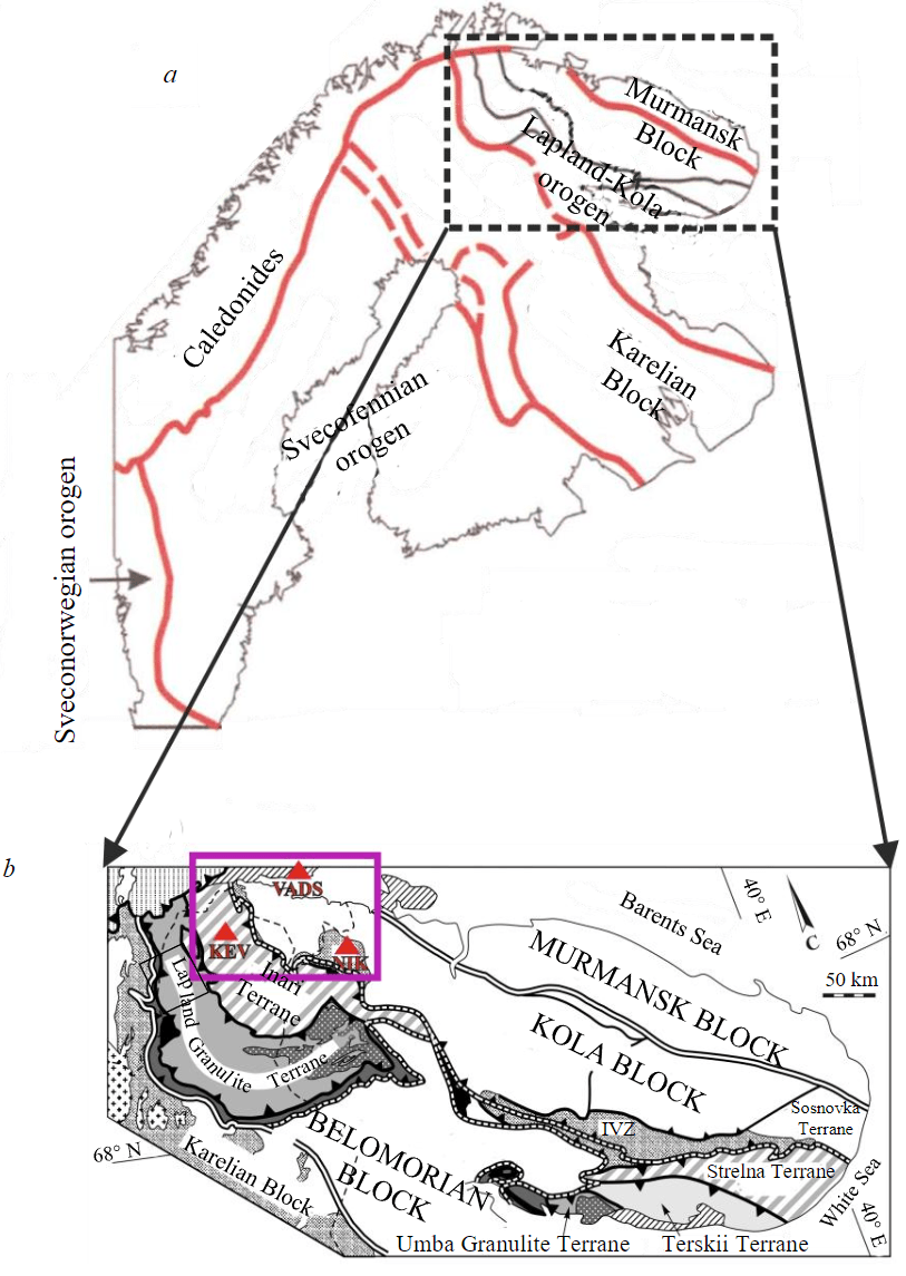
Fig.1. Tectonic sketch of the Fennoscandian Shield according to [3, 4] (a) and detailed tectonic map of the Kola region according to [4, 5] (b). Red triangles mark the positions of the seismic stations VADS, NIK, and KEV used in this work; the purple rectangle shows the study region
The article presents the results of new seismological studies regarding the northwestern LKO lithosphere structure. The Pechenga ore region and “Nikel” (NIK) seismic station located within it deserved our special attention. Researching this region’s structure may lead to solutions for a wide range of fundamental scientific issues. Additionally, Pechenga holds one of the largest sulphide copper-nickel deposits in the world, and its genesis is of major interest.
The initial studies of the Pechenga region’s deep structure began in 1960-1963 under the leadership of I.V.Litvinenko of the Leningrad Mining Institute, and used the method of deep seismic sounding along its Barents Sea – Pechenga – Lovno profile, and were later continued by many other scientists [15]. In addition, within the Pechenga region, a unique experiment on superdeep drilling of the SG-3 well (i.e. the Kola Superdeep Borehole) was carried out. The Earth’s crust was penetrated to a depth of 12,262 m, which allowed scientists to verify the results of indirect geophysical research with direct observations. As new data accumulated and the general understanding of the Earth’s evolution changed, the theories around the development of the Pechenga structure and the mineral deposits’ genesis have changed as well. According to the current scientific consensus, their genesis is attributed to Paleoproterozoic plumes that contributed to the rise of primitive magmas and undepleted material to the surface. Traces of these plumes can still be detected today [16, 17].
Methodology
To obtain deep velocity sections, the receiver function (RF) technique was used. It is based on the use of the converted phases of teleseismic waves forming at contrast seismic boundaries in a close proximity beneath a seismic station. These converted waves characterize the part of the medium in which they were formed. Thus, RF results can be effectively localized and interpreted by estimating the depth the converted waves formed at (conversion points).
The method is divided into two parts according to the types of converted phases used – the P-receiver function (or PRF), analyses P-S (Ps) converted waves and their multiples, and, accordingly, the S-receiver function (or SRF) analyses S-P (Sp) converted waves and their multiples. Joint inversion of PRF and SRF allows us to obtain a stable one-dimensional velocity section of the Earth’s crust and upper mantle [18, 19].
To obtain the receiver functions, we used a well-tested and reliable approach that is described in detail in [20]. Thus, we will discuss only the main aspects. The key elements of this methodology are as follows: at the first stage, we selected seismic events according to their epicentral distances; the criteria of epicentral distances for PRF analysis is 30-100°, while for SRF analysis it is 65-100°. The event parameters for this analysis (origin time, depth, and coordinates) were taken from the Global Centroid Moment Tensor Catalog (GCMT Catalog) [21, 22]. In addition, due to remote epicentral distances, earthquakes with a magnitude of less than 5.5 were not considered. We handpicked events with an impulse waveform of the first incident wave (P for PRF and S for SRF) and a high (more than 3) signal-to-noise ratio. The seismogram of each selected event was filtered (a second-order Butterworth filter with a corner period of 5 s was used to obtain PRF, and 8 s for SRF) and then their standard ZNE three-component coordinate system was rotated to a LQT ray coordinate system for PRF and LAB for SRF. In the LQT ray coordinate system, the L component coincides with the oscillation direction of the incident P wave, Q is perpendicular to L in the P-SV plane, and T is orthogonal to the LQ plane. In the LAB coordinate system, the L component corresponds to the direction of the movement of the incident wave, and A to the direction of polarization of the S wave. B is orthogonal to L and A. To standardize the recordings and minimize the influence of the focal mechanism, we applied deconvolution to each individual RF under the assumption that the L and A components in PRF and SRF are determined up to a normalizing factor by the shape of the incident wave and are near-independent of the medium parameters. During the deconvolution, we selected and applied to all components a filter that brings the observed waveforms on the L and A components closer to the gaussian shape.
To identify the converted phases that describe the seismic boundaries in the Earth's crust and upper mantle, the individual receiver functions we selected and prepared were stacked together. The stacking mechanisms for PRF and for SRF are different. For PRF, individual functions were stacked with adjustments that correspond to the beam parameter of a given incident wave and the depth of the conversion point. All events were reduced to the same beam parameter value – 6.4 s/deg. For each target depth and for each event, individual time corrections were estimated, by which the seismograms were shifted relative to each other before stacking. Stacked traces were estimated for multiple assumed conversion depths. The SRFs were stacked considering the weighting indices for the noise level on each of the traces and for the deviation of the incident S-wave polarization from the P-SV plane, as well as relative to the reference (usually average of all individual records’) epicentral distance. The method for estimating these indices is given in detail in [23].
To obtain deep velocity models, we carried out the joint inversion of PRF and SRF. The search for optimal models (minimization) was conducted using the Levenberg – Marquardt algorithm [24]. A model of the medium consisting of laterally homogeneous layers was used. The forward modelling of estimating synthetic receiver functions was done using the Thomson – Haskell matrix algorithm [25]. To obtain the required velocity models, a probabilistic-statistical approach was used with the generation of multiple random trial a priori models. The main advantage of this approach is independence from any initial velocity model.
In the given research, the varied parameters for the individual models were: the shear wave velocity Vs, the ratio of the primary and shear wave velocities Vp/Vs, and the thickness of each layer; the medium was set to consist of 14 layers. For the data from each seismic station, 100,000 random initial models and synthetic PRF and SRF were calculated, which were then minimized. The final velocity model was built as the median of a sample of 2-3 % of the best solutions (those synthetic PRFs and SRFs that best correlate with observations). To stabilize the inversion and estimate the absolute velocities along the section with increased precision, the converted waves’ travel time discrepancies from the boundaries of 410 and 660 km in the upper mantle relative to the IASP91 model (Δtp and Δts) [26] were also included in the inversion, which is demonstrated in [27]. To obtain the final distribution of varied parameters, the model parameter space was divided into cells. The solution is presented as a region saturated with minimized random initial models, where synthetic PRF and SRF best coincide with the observed data. The cells with the largest number of selected minimized trial models have been highlighted. The method used is described in detail in [28].
Data
As the data for this research, we used seismic recordings accumulated by the new NIK seismic station, which is located in the village of Nikel, Murmansk Region, near the largest copper-nickel deposits of the Pechenga region. The station was launched in 2020 and is equipped with a broadband velocimeter with a frequency range of 0.03-50 Hz and a RefTek 130 seismic recorder.
To assess the quality of the recordings obtained by the new NIK station, the levels of microseismic background noise were examined. To do this, we estimated the spectral noise power density SPM (Fig.2) based on the records of each of the components (Z, N, E) for the full set of continuous seismic data for the entire recording period; that data was compared to the permissible values for this parameter obtained during the observations of 75 “reference” seismic stations of the global network. The level of microseismic noise did not exceed the standard values in its entire registering range; moreover, the station can be classified as “quiet” when analyzing signals over up to 15 s periods.
In addition to the NIK station data, our research incorporates data from two other broadband seismic stations of the Global Network located in the northwestern part of the LKO – Vadso (VADS) and Kevo (KEV). Both stations are permanent and have been in operation for more than seven years. They are equipped with broadband velocimeters with a maximum recording period of at least 120 s, which ensures high quality of recorded seismic data. The main parameters of the seismic stations used are provided in the Table below.
Basic parameters of seismic stations and the number of estimated individual PRF and SRF receiver functions
|
Station code |
Station name |
Latitude |
Longitude |
Launch year |
Sensor type |
Bandwidth, Hz |
PRF |
SRF |
|
NIK |
Nikel |
69.24 |
30.13 |
2020 |
RefTek 151-30 |
0.03-50 |
41 |
32 |
|
VADS |
Vadso |
70.12 |
29.36 |
2016 |
Trillium 120 PA |
0.008-30 |
85 |
143 |
|
KEV |
Kevo |
69.75 |
27.00 |
1993 |
STS 1 |
0.002-10 |
247 |
200 |
Based on the analyzed seismic data, 143 individual SRFs and 85 individual PRFs were obtained from the VADS station; from the KEV station – 200 SRFs, 247 PRFs; from the NIK station – 32 SRFs, 41 PRFs. The distribution of epicentres for the selected events is shown in Fig.3. The distribution of the epicentres for the selected events makes it possible to avoid azimuthal dependence when obtaining velocity models after stacking individual PRFs and SRFs. That is also true for the NIK station, which has the lowest amount of accumulated data. The azimuth values in degrees are plotted along the perimeter of the grid, and the epicentral distances in degrees are plotted along the azimuthal directions.
Results
The receiver function method is characterised by high sensitivity to seismic velocity contrasts and relatively low accuracy when it comes to absolute velocity estimates. This issue can be resolved by using the values of the detected travel time discrepancies of the converted waves formed at the boundaries of the phase transition zone in the upper mantle at depths of about 410 and 660 km [27]. In addition, the presence of well-defined phases from these global boundaries in the recordings is an additional marker of high-quality experimental data. To determine the observed discrepancies using the PRF data for each station, we constructed stacks in accordance with the methodology described above (Fig.4).
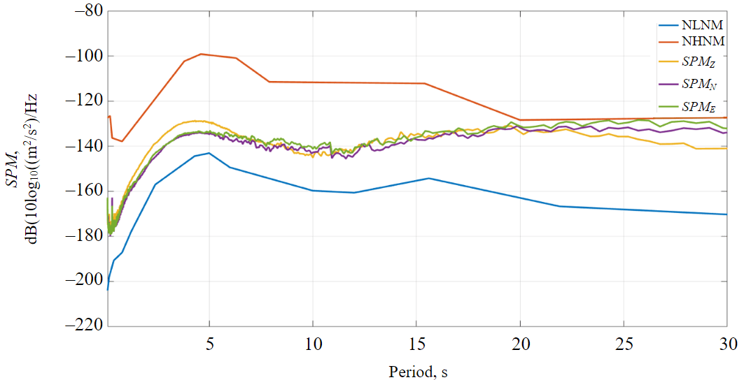
Fig.2. Noise power spectral density for each of the component (SPMZ, SPMN, SPME) for the NIK station data. NLNM and NHNM – minimum and maximum permissible values of this parameter
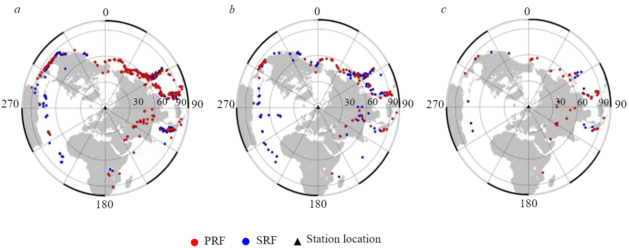
Fig.3. Epicenters of seismic events for PRF and SRF for KEV (a), VADS (b) and NIK (c) stations
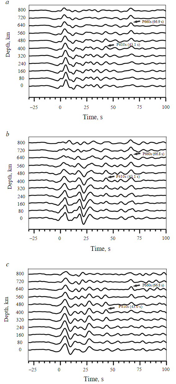
Fig.4. Stacks of PRF records for KEV (a), VADS (b), and NIK (c) stations (the observed delay times of the maximum amplitudes of converted waves relative to the arrival time of the first P-wave are indicated in parentheses; the target conversion depth is indicated for each trace)
The analyzed Ps converted waves from the P410s and P660s mantle transition zone boundaries are easily observable in the stacks. Moreover, these phases are “focusing” at appropriate depths, i.e. the maximum phase amplitude is observed on the stack corresponding to the expected depth (400 km stack for 410 km discontinuity and 640 km stack for 660 km discontinuity). For each individual station, consistent values (with approximately a 0.1 s margin of error) of the arrival times of these phases were obtained. According to the standard IASP91 Earth velocity model and a ray parameter of 6.4 s/deg, to which the selected recordings are reduced, P410s and P660s phases should be registered at 44 and 67.9 s. The resulting data, however, indicates consistent negative time discrepancies tobs – tstd = –1 both for the P410s and P660s phases, which in turn indicates average increased velocities in the upper mantle.
Based on joint PRF and SRF modelling and observed discrepancies in the travel times of converted P410s and P660s waves, we obtained velocity models of the Earth’s crust and upper mantle to a depth of about 300 km for each individual station (Fig.5). The most significant identified feature of the upper mantle structure is a layer of relatively low velocities for the VADS station at depths of 140-170 km. In the same interval, a low velocity layer is also observed at the KEV station, but it is significantly less pronounced. For the NIK station data, the low velocity layer is not observed.
The velocity structure of the Earth's crust within the research area does not reveal any common distinguishable features or seismic boundaries of high contrast (Fig.6). The average velocity values in the crust calculated using VADS station data are significantly higher than both the values of the standard IASP91 Earth velocity model and those observed at the KEV and NIK stations. However, a significant difference in the crust-mantle transition structure is apparent. According to the VADS station model, it appears as a well-defined boundary at a depth of about 46 km, while for KEV station the model around this depth shows a relatively smooth velocity gradient and velocity values reaching standard values for the mantle at a depth of about 55 km. In the NIK model, two boundaries are identifiable in the lower crust at depths of 37 and 47 km; moreover, the modelled velocities match a standard mantle at a depth of about 47 km, which makes it preferable for determining the depth of the Moho.
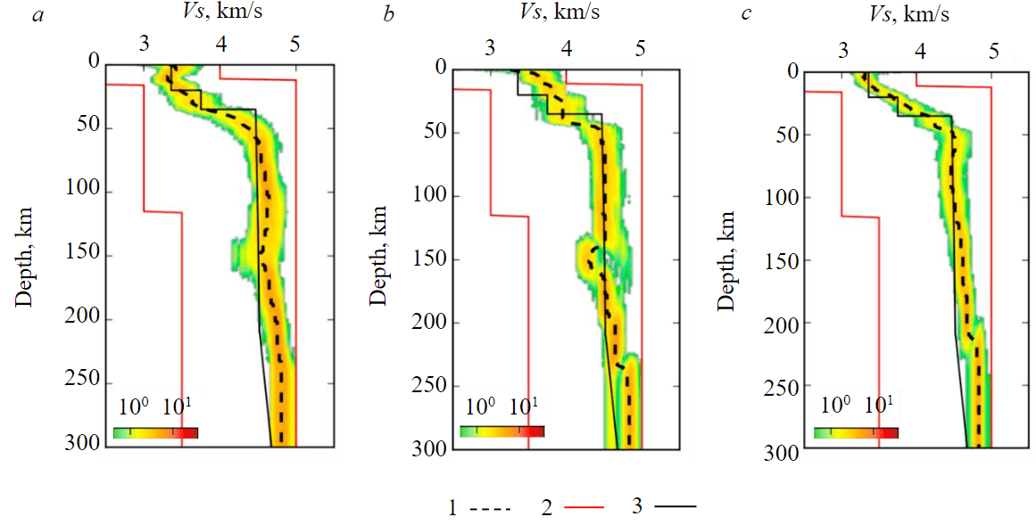
Fig.5. Shear wave velocity models to depths of about 300 km for KEV (a), VADS (b) and NIK (c) stations (conden-sation fields of individual minimized trial models) 1 – final median models; 2 – the boarders of the formation of trial initial models; 3 – IASP91 model
Discussion
Despite the stations being in relatively close proximity, the obtained velocity models indicate that the lithosphere velocity structures in the northwestern part of the LKO vary significantly. Moreover, differences can be traced not only in the crustal structure, but in the upper mantle as well. The consistency of results across all stations is achieved using structural features analysis for the 410 and 660 km boundaries.
Based on the Vs distribution model, obtained for the VADS station, we observe a low-velocity layer in the upper mantle at depths of 140-170 km. The KEV station reveals a decrease in seismic velocities at the indicated depths as well; however, it is not easily identifiable and it is impossible to reliably confirm or deny the presence of a low-velocity layer for this station. The relatively shallow depths (about 140-170 km) at which this layer was discovered do not allow us to associate it with the asthenosphere [29]. It is possible that our models marked the mid-lithosphere discontinuity or MLD. The presence of this layer in various regions of the Earth, including the Fennoscandian Shield, was first described using seismic data in [30]. This layer appears to be global, at least for craton areas. However, its depth, thickness, and seismic velocities vary within different tectonic structures and probably depend on local geological history [31-33]. It is worth noting that for most regions of the Earth, this layer is characteristically present at the depth range of 100-150 km, including for the central and eastern parts of the Kola region. Analyzing data obtained by the “Kvartz” superlong profile conducted using peaceful nuclear explosions, the presence of the low-velocity layer is shown at the depths of about 80-140 km [34]. For Finland, seismic tomography data has identified a low-velocity layer with parameters, which differ for the northern and southern parts of the territory. In particular, its depth was shown to increase in a northerly direction. [35]. In the area where the KEV station was installed, the low-velocity layer was observed at a depth of about 180 km, which does not contradict our estimates, considering the greater accuracy of RF at those depths.
At present, there is no model describing the formation mechanism and nature of mid-lithospheric discontinuity (MLD). Among the hypotheses expressed, the following can be distinguished: rheolo-gical – layering at a temperature close to the solidus point [36]; petrophysical – layering under conditions of either partial submergence of the substance [37] or in the presence of basaltic melts [36, 38]; change in deformation properties with depth [39].
Dissimilarities in the depth and character of the crust-mantle transition cannot be unambiguously interpreted using models obtained from the KEV, VADS, and NIK stations, as data from three seismic stations is not sufficient to provide a complete understanding on a regional level. In order to significantly alter the Moho structure, a large-scale tectonic process is required. It would be most logical to associate with Caledonian orogen formation artifacts, developed as a result of the collision of the Baltica-Avalonia-Laurentia microcontinents [40, 41]. The change in the sharpness of the Moho can be associated with reorganisation during deformation, which possibly led to dissolution of the high-velocity layer within the lower crust that is found in central and southern Sweden [42] (and which may have been metamorphosized into eclogites, locally found on the surface along the coast of Norway).
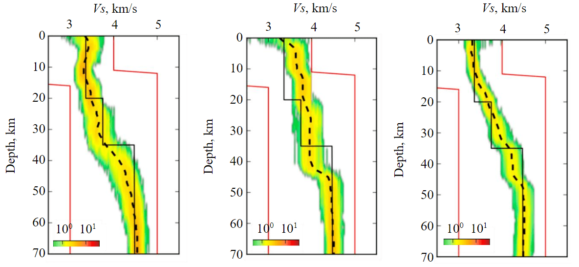
Fig.6. Shear wave velocity models to depths of about 70 km for KEV (a), VADS (b) and NIK (c) stations (for symbols, see Fig.5)
Of greatest interest is the deep structure model of the Pechenga region obtained using the new NIK seismic station data (Fig.7). It is located in close proximity to the major copper-nickel deposits of Kotselvaara-Kammikivi and the Zhdanovskii eastern ore cluster, and 42 km from the SG-3 Kola Superdeep Borehole.
In the resulting NIK Earth's crust velocity structure model, contrasting seismic boundaries are not detected. In the lower part of both the Vp and Vs velocity section, two seismic boundaries are observed at the depths of 37 and 47 km, respectively. The velocity values match the standard for the upper mantle at the depths of about 47 km. The complex two-stage structure of the crust-mantle transition with two boundaries – M1 and M2, is generally confirmed by other geophysical methods [43, 44]. Such “splitting” of the crust-mantle transition can be interpreted as a large-scale tectonic process relic, for example, a mantle diapir or plume, which is believed to have existed in the Pechenga region in the Proterozoic [16]. It should be noted that traces of mantle diapirs in the modern geological structure have been found in various regions of the Earth (for example, in the Russian Far East [45]).
Another distinct feature of the new depth models obtained is the anomalously high Vp/Vs parameter (~ 2) zone, which is observed from the surface to the depth of about 20 km. Velocity models obtained by the RF method can be spatially localized for a given depth. To determine a region that is characterized by velocity patterns, conversion points can be estimated, i.e. projections of converted wave formation points onto the surface for a given depth. Fig.7 shows the conversion points for a depth of 20 km and outlines the area characterized by the resulting velocity models for the given depth. The presence of a zone with such a high Vp/Vs ratio within the Earth’s crust may indicate not only a preserved intermediate magma chamber [46], which may contain ore mineralization, but also the preservation of a relict magma channel through which the material reached the surface.
Direct comparison between the velocity sections obtained in this research and the results of SG-3 studies is complicated for a number of reasons. This is primarily due to the long-period nature of the data used in the RF technique, which leads to significant lateral averaging, which does not allow us to distinguish layers several hundred metres thick, which were observed during the Kola superdeep well experiment [47]. In addition, the SG-3 research provided significantly more accurate Vp velocities, while the RF method is more focused on determining Vs. It should be noted that the seismic velocities obtained by the author are in qualitative agreement with the values shown in the SG-3 section and with modern spatial regional tomographic models of the Pechenga region [43, 47].
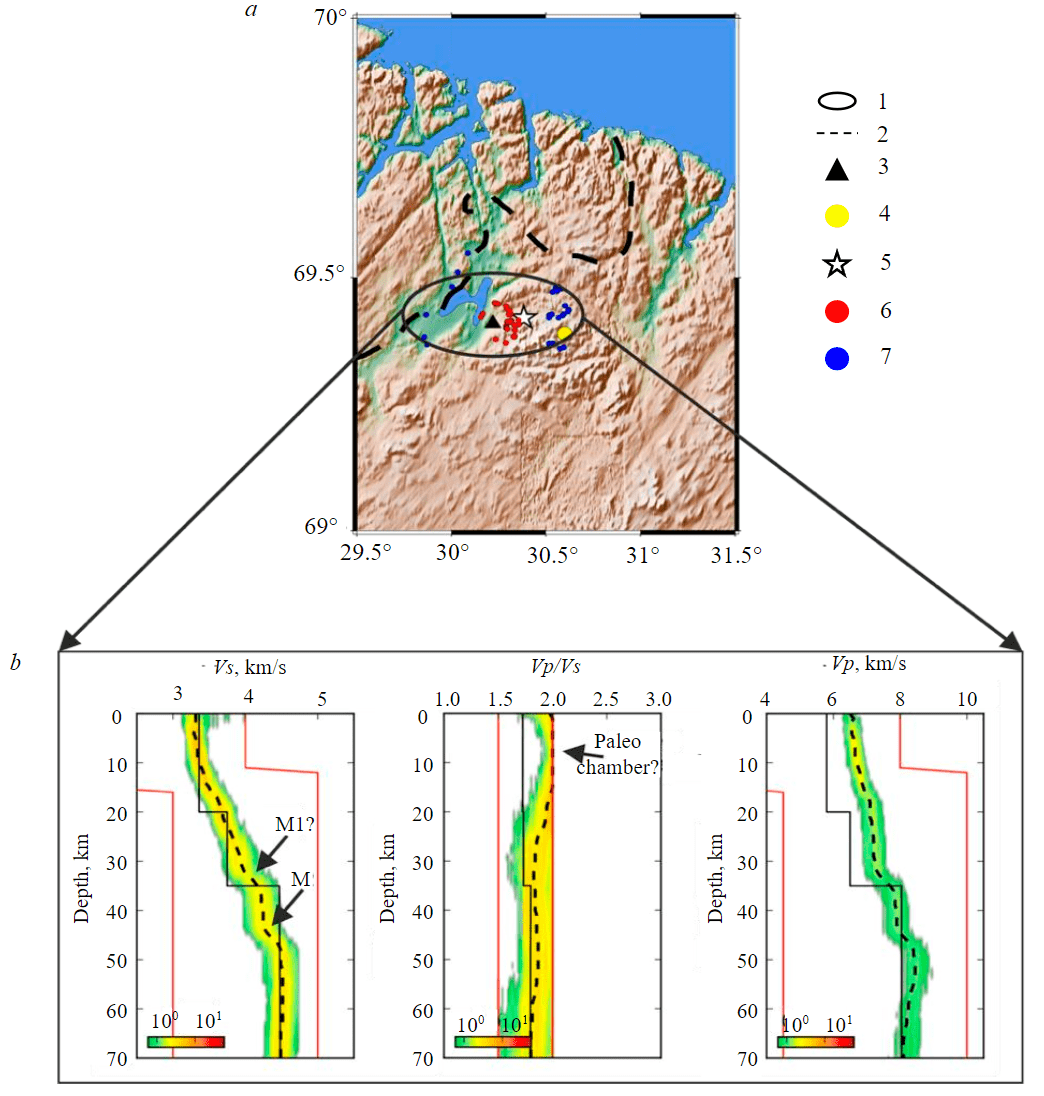
Fig.7. Map of the Pechenga region (a) and velocity models (b) of Vs, Vp/Vs, and Vp with depth (for symbols, see Fig.5) 1 – area characterized by velocity models at the depth of about 20 km; 2 – state border; 3 – NIK seismic station; 4 – Kola superdeep well; 5 – Kaula-Kotselvaara mine; 6 – PRF conversion points for a depth of 20 km; 7 – SRF conversion points for a depth of 20 km
Conclusion
Seismological data from three seismic stations located in the northwestern part of the Lapland-Kola orogen was analyzed. Two of these stations are well established, KEV in northern Finland and VADS in the northeastern part of the Norwegian Caledonides, joining them in 2020 was the NIK station, established in the Pechenga ore region. As part of the research, it was shown that the lithosphere in the research area has a heterogeneous velocity structure not only within the Earth’s crust, but also in the upper mantle, to a depth of approximately 200 km. In the upper mantle structure, a zone of lower velocities can be traced at depths of about 150 km, most likely associated with mid-lithospheric discontinuity. MLD is most clearly manifested in northern Finland, hardly observable beneath the Norwegian Caledonides, and is not observed beneath the Pechenga region. Significant differences were revealed in the structure of the crust-mantle transition, represented by a single discontinuity at a depth of 46 km (VADS station), a gradient layer with seismic wave velocities reaching standard values for the mantle at a depth of about 55 km (KEV station), and a complex zone with two boundaries at the depths of about 37 and 47 km beneath the Pechenga region (NIK station). Considering the absolute values of velocities, the lower boundary detected at the NIK station looks preferable for detecting the Moho.
The Pechenga region model indicates the presence of anomalously high values of the Vp/Vs ratio (~ 2) from the surface to depths of about 20 km in the area of the major copper-nickel deposits of Kotselvaara-Kammikivi and the Zhdanovskii eastern ore cluster. Such high values are indicative, in particular, of undepleted mantle rocks, and may be associated with an intermediate magma chamber relic formed during the Proterozoic rifting.
The identified anomalies in the structure of the crust-mantle transition, Vp/Vs values, as well as the absence of MLD beneath the Pechenga region (its presence was shown in the neighbouring areas) can be jointly interpreted as artifacts of the Proterozoic plume magmatism stage, characteristic of the Pechenga region and confirmed by geological and geochemical research [16].
References
- Daly J.S., Balagansky V.V., Timmerman M.J., Whitehouse M.J. The Lapland–Kola orogen: Palaeoproterozoic collision and accretion of the northern Fennoscandian lithosphere. European Lithosphere Dynamics: Geological Society Memoirs. London: Geological Society. 2006. Vol. 32, p. 579-598. DOI: 10.1144/GSL.MEM.2006.032.01.35
- Hjelt S.-E., Daly J.S. SVEKALAPKO colleagues. SVEKALAPKO: evolution of Palaeoproterozoic and Archaean Lithosphere. Lithosphere Dynamics: Origin and Evolution of Continents. Uppsala: EUROPROBE Secretariat, Uppsala University, 1996, p. 56-67.
- Gorbatschev R., Bogdanova S. Frontiers in the Baltic Shield. Precambrian Research. 1993. Vol. 64. Iss. 1-4, p. 3-21. DOI: 10.1016/0301-9268(93)90066-B
- Mudruk S.V., Balagansky V.V., Gorbunov I.A., Raevsky A.B. Alpine-type tectonics in the Paleoproterozoic Lapland-Kola Orogen. Geotectonics. 2013. Vol. 47. N 4, p. 251-265. DOI: 10.1134/S0016852113040055
- Balagansky V.V., Glaznev V.N., Osipenko L.G. Early Proterozoic evolution of the northeastern Baltic Shield: terrane analysis. Geotectonics. 1998. Vol. 32. N 2, p. 81-93.
- Amelin Y.V., Semenov V.S. Nd and Sr isotopic geochemistry of mafic layered intrusions in the eastern Baltic shield: implications for the evolution of Paleoproterozoic continental mafic magmas. Contributions to Mineralogy and Petrology. 1996. Vol. 124. Iss. 3-4, p. 255-272. DOI: 10.1007/s004100050190
- Lobach-Zhuchenko S.B., Arestova N.A., Chekulaev V.P. et al. Geochemistry and petrology of 2.40-2.45 Ga magmatic rocks in the north-western Belomorian Belt, Fennoscandian Shield, Russia. Precambrian Research. 1998. Vol. 92. Iss. 3, p. 223-250. DOI: 10.1016/S0301-9268(98)00076-X
- Sharkov E.V., Bogatikov O.A., Krasivskaya I.S. The Role of Mantle Plumes in the Early Precambrian Tectonics of the Eastern Baltic Shield. Geotectonics. 2000. Vol. 34. N 2, p. 85-105.
- Williams H., Hoffman P.F., Lewry J.F. et al. Anatomy of North America: thematic geologic portrayals of the continent. Tectonophysics. 1991. Vol. 187. Iss. 1-3, p. 117-134. DOI: 10.1016/0040-1951(91)90416-P
- Pesonen L.J., Elming S.-Å., Mertanen S. et al. Palaeomagnetic configuration of continents during the Proterozoic. Tectonophysics. 2003. Vol. 375. Iss. 1-4, p. 289-324. DOI: 10.1016/S0040-1951(03)00343-3
- Mints M.V., Konilov A.N. Geodynamic crustal evolution and long-lived supercontinents during the Palaeoproterozoic: evidence from granulite-gneiss belts, collisional and accretionary orogens. The Precambrian Earth, Tempos and Events. Elsevier, 2004. Vol. 12. P. 223-239.
- Balaganskii V.V., Mints M.V., Deili Dzh.S. Paleoproterozoic Lapland-Kola orogeny. Structure and dynamics of the lithosphere in Eastern Europe. Results of research under the EUROPROBE program. Moscow: GEOKART; GEOS, 2006. Vol. 2, p. 158-171 (in Russian).
- Daly J.S., Balagansky V.V., Timmerman M.J. et al. Ion microprobe U–Pb zircon geochronology and isotopic evidence for a trans-crustal suture in the Lapland–Kola Orogen, northern Fennoscandian Shield. Precambrian Research. 2001. Vol. 105. Iss. 2-4, p. 289-314. DOI: 10.1016/S0301-9268(00)00116-9
- Lahtinen R., Huhma H. A revised geodynamic model for the Lapland-Kola Orogen. Precambrian Research. 2019. Vol. 330, p. 1-19. DOI: 10.1016/j.precamres.2019.04.022
- Sharov N.V. Lithosphere of Northern Europe: seismic data. Petrozavodsk: Karelian Research Centre, RAS, 2017, p. 173 (in Russian).
- Skufin P.K., Bayanova T.B. Early Proterozoic central-type volcano in the Pechenga structure and its relation to the ore-bearing gabbro-wehrlite complex of the Kola Peninsula. Petrology. 2006. Vol. 14. N 6, p. 609-627. DOI: 10.1134/S0869591106060063
- Arzamastsev A.A., Salnikova E.B., Stepanova A.V. et al. Mafic Magmatism of Northeastern Fennoscandia (2.06–1.86 Ga): Geochemistry of Volcanic Rocks and Correlation with Dike Complexes. Stratigraphy and Geological Correlation. 2020. Vol. 28. N 1, p. 3-40. DOI: 10.1134/S0869593820010025
- Kosarev G.L., Oreshin S.I., Vinnik L.P. et al. Heterogeneous lithosphere and the underlying mantle of the Indian subcontinent. Tectonophysics. 2013. Vol. 592, p. 175-186. DOI: 10.1016/j.tecto.2013.02.023
- Oreshin S., Kiselev S., Vinnik L. et al. Crust and mantle beneath western Himalaya, Ladakh and western Tibet from integrated seismic data. Earth and Planetary Scientific Letters. 2008. Vol. 271. Iss. 1-4, p. 75-87. DOI: 10.1016/j.epsl.2008.03.048
- Vinnik L.P. Receiver Function Seismology. Izvestiya, Physics of the Solid Earth. 2019. Vol. 55. N 1, p. 12-21. DOI: 10.1134/S1069351319010130
- Dziewonski A.M., Chou T.-A., Woodhouse J.H. Determination of earthquake source parameters from waveform data for studies of global and regional seismicity. Journal of Geophysical Research: Solid Earth. 1981. Vol. 86. Iss. B4, p. 2825-2852. DOI: 10.1029/JB086iB04p02825
- Ekström G., Nettles M., Dziewonski A.M. The global CMT project 2004-2010: Centroid-moment tensors for 13,017 earthquakes. Physics of the Earth and Planetary Interiors. 2012. Vol. 200-201, p. 1-9. DOI: 10.1016/j.pepi.2012.04.002
- Farra V., Vinnik L. Upper mantle stratification by P and S receiver functions. Geophysical Journal International. 2000. Vol. 141. Iss. 3, p. 699-712. DOI: 10.1046/j.1365-246x.2000.00118.x
- Press W.H., Teukolsky S.A., Vetterling W.T., Flannery B.P. Numerical Recipes: The Art of Scientific Computing. New York: Cambridge University Press, 2007, p. 1256.
- Haskell N.A. Crustal reflection of plane P and SV waves. Journal of Geophysical Research. 1962. Vol. 67. N 12, p. 4751-4768. DOI: 10.1029/JZ067i012p04751
- Kennett B.L.N., Engdahl E.R. Traveltimes for global earthquake location and phase identification. Geophysical Journal International. 1991. Vol. 105. Iss. 2, p. 429-465. DOI: 10.1111/j.1365-246X.1991.tb06724.x
- Vinnik L., Kozlovskaya E., Oreshin S. et al. The lithosphere, LAB, LVZ and Lehmann discontinuity under central Fennoscandia from receiver functions. Tectonophysics. 2016. Vol. 667, p. 189-198. DOI: 10.1016/j.tecto.2015.11.024
- Aleshin I.M. The inverse problem solution with an ensemble of models: an example for receiver function inversion. Doklady Earth Sciences. 2021. Vol. 496. N 1, p. 63-66. DOI: 10.31857/S2686739721010047
- Wang Z., Kusky T.M. The importance of a weak mid-lithospheric layer on the evolution of the cratonic lithosphere. Earth-Science Reviews. 2019. Vol. 190, p. 557-569. DOI: 10.1016/j.earscirev.2019.02.010
- Thybo H., Perchuć E. The Seismic 8° Discontinuity and Partial Melting in Continental Mantle. Science. 1997. Vol. 275. Iss. 5306, p. 1626-1629. DOI: 10.1126/science.275.5306.1626
- Yang H., Artemieva I.M., Thybo H. The Mid-Lithospheric Discontinuity Caused by Channel Flow in Proto-Cratonic Mantle. Journal of Geophysical Research: Solid Earth. 2023. Vol. 128. Iss. 4. N e2022JB026202. DOI: 10.1029/2022JB026202
- Weijia Sun, Li-Yun Fu, Erdinc Saygin, Liang Zhao. Insights Into Layering in the Cratonic Lithosphere Beneath Western Australia. Journal of Geophysical Research: Solid Earth. 2018. Vol. 123. Iss. 2, p. 1405-1418. DOI: 10.1002/2017JB014904
- Rychert C.A., Shearer P.M. A Global View of the Lithosphere-Asthenosphere Boundary. Science. 2009. Vol. 324. Iss. 5926, p. 495-498. DOI: 10.1126/science.1169754
- Yegorova T.P., Pavlenkova G.A. Velocity–Density Models of the Earth’s Crust and Upper Mantle from the Quartz, Craton, and Kimberlite Superlong Seismic Profiles. Izvestiya, Physics of the Solid Earth. 2015. Vol. 51. N 2, p. 250-267. DOI: 10.1134/S1069351315010048
- Silvennoinen H., Kozlovskaya E., Kissling E. POLENET/LAPNET teleseismic P wave travel time tomography model of the upper mantle beneath northern Fennoscandia. Solid Earth. 2016. Vol. 7. Iss. 2, p. 425-439. DOI: 10.5194/se-7-425-2016
- Thybo H. The heterogeneous upper mantle low velocity zone. Tectonophysics. 2006. Vol. 416. Iss. 1-4, p. 53-79. DOI: 10.1016/j.tecto.2005.11.021
- Yuan H., Romanowicz B. Lithospheric layering in the North American craton. Nature. 2010. Vol. 466. Iss. 7310, p. 1063-1068. DOI: 10.1038/nature09332
- Rader E., Emry E., Schmerr N. et al. Characterization and Petrological Constraints of the Midlithospheric Discontinuity. Geochemistry, Geophysics, Geosystems. 2015. Vol. 16. Iss. 10, p. 3484-3504. DOI: 10.1002/2015GC005943
- Shun-ichiro Karato, Olugboji T., Park J. Mechanisms and geologic significance of the mid-lithosphere discontinuity in the continents. Nature Geoscience. 2015. Vol. 8. N 7, p. 509-514. DOI: 0.1038/ngeo2462
- Corfu F., Gasser D., Chew D.M. New perspectives on the Caledonides of Scandinavia and related areas: introduction. New Perspectives on the Caledonides of Scandinavia and Related Areas. London: Geological Society, 2014. Special Publications. Vol. 390, p. 9-43. DOI: 10.1144/SP390.28
- Egorov A.S., Vinokurov I.Yu., Telegin A.N. Scientific and Methodical Approaches to Increase Prospecting Efficiency of the Russian Arctic Shelf State Geological Mapping. Journal of Mining Institute. 2018. Vol. 233, p. 447-458. DOI: 10.31897/PMI.2018.5.447
- Buntin S., Artemieva I.M., Malehmir A. et al. Long-lived Paleoproterozoic eclogitic lower crust. Nature Communications. 2021. Vol. 12. N 6553. DOI: 10.1038/s41467-021-26878-5
- Isanina E.V. The receiver function method (from the earthquake – RFM) investigations on the SD-3 district. Apatity: Kola Science Centre Russian Academy of Science, 1997, p. 101-115 (in Russian).
- Sharov N.V., Isanina E.V., Krupnova N.A. Deep structure of the Kola Superdeep Borehole area (from seismic data). Vestnik of MSTU. 2007. Vol. 10. N 2, p. 309-319 (in Russian).
- Alekseev V.I. Deep structure and geodynamic conditions of granitoid magmatism in the Eastern Russia. Journal of Mining Institute. 2020. Vol. 243, p. 259-265. DOI: 10.31897/PMI.2020.3.259
- Lobanov K.V., Chicherov M.V., Chizhova I.A. et al. Depth structure and ore-forming systems of the Pechenga ore region (Russian Arctic Zone). Arctic: Ecology and Economy. 2019. N 3 (35), p. 107-122 (in Russian). DOI: 10.25283/2223-4594-2019-3-107-122
- Kola Superdeep. Scientific Results and Research Experience. Moscow: “TECHNONEFTEGAZ”, 1998, p. 260 (in Russian).