
Investigation of probabilistic models for forecasting the efficiency of proppant hydraulic fracturing technology
- 1 — Ph.D., Dr.Sci. Perm National Research Polytechnic University ▪ Scopus ▪ ResearcherID
- 2 — Engineer Branch of LLC LUKOIL-Engineering PermNIPIneft in the city of Perm ▪ Orcid ▪ Elibrary ▪ Scopus

Abstract
To solve the problems accompanying the development of forecasting methods, a probabilistic method of data analysis is proposed. Using a carbonate object as an example, the application of a probabilistic technique for predicting the effectiveness of proppant hydraulic fracturing (HF) technology is considered. Forecast of the increase in the oil production of wells was made using probabilistic analysis of geological and technological data in different periods of HF implementation. With the help of this method, the dimensional indicators were transferred into a single probabilistic space, which allowed performing a comparison and construct individual probabilistic models. An assessment of the influence degree for each indicator on the HF efficiency was carried out. Probabilistic analysis of indicators in different periods of HF implementation allowed identifying universal statistically significant dependencies. These dependencies do not change their parameters and can be used for forecasting in different periods of time. Criteria for the application of HF technology on a carbonate object have been determined. Using individual probabilistic models, integrated indicators were calculated, on the basis of which regression equations were constructed. Equations were used to predict the HF efficiency on forecast samples of wells. For each of the samples, correlation coefficients were calculated. Forecast results correlate well with the actual increase (values of the correlation coefficient r = 0.58-0.67 for the examined samples). Probabilistic method, unlike others, is simple and transparent. With its use and with careful selection of wells for the application of HF technology, the probability of obtaining high efficiency increases significantly.
None
Introduction
Time series forecasting is one of the most common forms for the statement of the forecasting problem, the solution of which plays an essential role in the strategic planning processes. Application of the currently existing mathematical models and methods for forecasting time series is closely related to the specifics of the subject area. The problem of time series forecasting is solved on the basis of creating a forecasting model that adequately describes the process under study.
Considered class of time series with regular constant components is used in subject areas, in which the influence of various factors is significant. An example of such a sphere is the oil industry, where the profit of a company or a country depends on confidence in the fulfillment of plans for oil production. Fulfillment of plans for oil production depends on many factors: technological, due to the technology of oil production; technical, depending on the applied technical means for intensifying oil production and geological, due to the structure of the space where the residual oil reserves are located. To predict the dynamics of the well operation [17, 18, 21], a set of geological and physical factors characterizing the reserve or the region of the well are used. In the presence of time series for this class in different areas, solving the forecasting problem is an important scientific and technical problem.
As of 01.01.2020, the following statistical and structural models for time series forecasting have been developed and applied: regression forecasting models [6, 9-11]; models using genetic algorithms [3]; model based on neural networks [4, 14, 15]; on classification and regression trees [1]; based on Markov processes [13]; based on clustering [5, 8]; based on self-organizing maps (Kohonen maps) [2]; based on fuzzy logic [7, 12]; on Bayesian networks [13].
All statistical and structural time series forecasting models have advantages and disadvantages.
Regression models and methods. Advantages of these models include the simplicity, flexibility, and uniformity of their analysis. Using linear regression models, the forecast result can be obtained faster than using other models. In addition, the transparency of the modeling is an advantage; i.e., the availability for analysis of all intermediate calculations. The main disadvantage of non-linear regression models is the complexity of determining the type of functional dependence, as well as the complexity of determining the main parameters of the model involved in the calculations.
Neural network models and methods. The main advantage of neural network models is non-linearity, i.e. the ability to establish non-linear relationships between future and actual values of processes. Other important advantages include adaptability, scalability, and consistency in analysis and design. Disadvantages are the lack of transparency in modeling, complexity of the architecture choice, high requirements for the consistency of the tutoring sample, choice complexity of the tutoring algorithm and the resource intensity of the tutoring process.
Models based on classification-regression trees. Advantages of the models in this class are: scalability (due to which fast processing of extremely large amounts of data is possible), speed and unambiguity of the tree learning process, as well as the possibility of using categorical external factors. Disadvantages are ambiguity of the algorithm for constructing the tree structure and the complexity of determining the moment to stop further branching.
It is not possible to judge the forecasting accuracy of the given forecasting models. Accuracy of forecasting a particular process depends not only on the model, but also on the experience of the researcher, on how well he understood the structure of a particular forecasting model, on the availability of data, and many other factors. However, the main disadvantages of existing forecasting methods can be grouped: a large number of free parameters requiring identification; various units used in forecasting indicators; unavailability of intermediate calculations performed in the “black box”; the complexity of assessing the individual influence degree of the indicators used on the output value. Thus, it is often difficult to determine which indicators have the greatest impact on the output and to rank them.
The task of forecasting time series is relevant for many subject areas and is an important part of the daily work of the “LUKOIL-Perm” LLC enterprises. To solve these problems, it is proposed to consider the possibilities of using the probabilistic method, which is described in sufficient detail in [16, 19, 22, 23]. In this work, a forecast of an increase in oil production is made using a probabilistic method for analyzing geological and technological data on the example of the experience of using proppant HF technology at the B3B4 carbonate object (upper Carboniferous sediments). Geological and technological parameters of wells are known at the selection stage, which allows making calculations of the technology efficiency in advance and give recommendations for its implementation.
As of 01.01.2019, 66 proppant HF operations were performed at the В3В4 site with an average initial increase in oil production of 7.1 tons/day. Let us divide the pool of wells into two classes: class I with increase in oil production > 7 tons/day – technology is effective, class II with increase in oil production < 7 tons/day – technology is ineffective. Initially, for each class of wells in the studied development sites, a statistical analysis of more than 50 indicators was performed. As a result of the analysis, parameters have been established that affect the efficiency of proppant HF. Importance of indicators was assessed by comparing the average values in the two classes according to the criterion of information content
where X1, X2 – average values of indicators for wells of classes I and II; – variance of indicators.
Criterion tp made it possible to reduce the initially available number of indicators to several.
Main geological and technological indicators:
- Geological parameters: coefficients of porosity mpor, %; productivity Kprod, m3/day∙MPa; near-bottomhole zone permeability , μm2; remote-bottomhole zone permeability , μm2; piezoconductivity γ, cm2∙s; skin factor S; gamma log values GK, μr/h; neural-gamma gamma log values NGK, μr/h; drilled-in net oil thickness hn, m; relative depth formation Hrel, m; absolute Habs, m.
- Technological parameters: current formation pressure in the well Рf, MPa; cumulative oil production since the beginning of well operation Qoil.c, tons; water production Qw.c, tons.
It is proposed to perform probabilistic data analysis and build probabilistic models based on geological and technological indicators of wells formed in the periods: 2014-2015 (20 wells); 2014-2016 (29 wells); 2014-2017 (50 wells); 2014-2018 (66 wells).
Initially, it is planned to build a probabilistic model for wells in 2014-2015, i.e., each geological and technological parameter N, which has a dimension (MPa, μm2, tons, etc.), is converted into a dimensionless value. Converting dimensional values into dimensionless ones will allow comparing indicators in a single probability space with each other. Based on the analysis results for each indicator, a probabilistic equation is constructed:
Probabilistic equation will make it possible to determine the criteria for the application of HF technology and rank the indicators according to the degree of influence on the actual increase in oil production . We will consider an increase in oil production rate of 7 tons/day achievable if the probability 0.5 units, this value will be the minimum criterion for the technology application. Degree of influence is defined as the difference between the maximum and minimum values of P(N). Following the analysis, it is planned to add nine wells of 2016 and perform a characteristics analysis. With the addition of new wells to the sample (2016-2018), the probabilistic models are recalculated, changes in the B coefficient are analyzed, and the criteria for the technology application change.
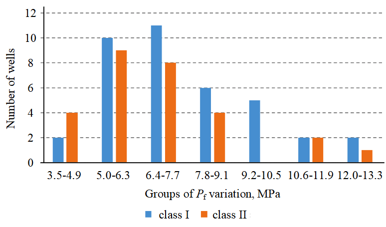
Fig.1. Histogram of the dependence for the number of well on groups of formation pressure variation Pf
Let us consider the methodology for constructing individual probabilistic models using the example of the current formation pressure in the well Pf. Average indicator values for wells where HF technology is effective and ineffective differ by 1.1 times. Average value in class I Pf = 7.7 MPa, in class II Pf = 6,8 MPa. Further, using this characteristic, distribution densities of the two classes under study were investigated. In the first case, data on class I values are studied, n1 = 38, in the second case – data on class II, n2 = 28.
Following the methodology used, at the first stage of constructing a probabilistic model based on the Pf indicator for classes I and II, a histogram is constructed. Optimal values of the intervals for values of the indicator Pf are calculated by the Sturgess formula:
To study the ratios for the proportion of values that fell into different intervals of variation of Pf, an interval analysis was performed (Fig.1).
At the next step, probability of the group belonging to the class is calculated:
where Ng – number of cases for Pf belonging to a group; Nk – sample volume for classes I and II.
Calculation results are presented in Table 1.
Table 1
Distribution of probability values P(Pf) of groups belonging to classes
|
Wells |
Variation intervals for formation pressure Pf, cm2/s |
|||||
|
3.5-4.9 |
5.0-6.3 |
6.4-7.7 |
7.8-9.1 |
9.2-10.5 |
10.6-11.9 |
|
|
Class I at n1 = 38 |
0.053 |
0.263 |
0.289 |
0.158 |
0.132 |
0.053 |
|
Class II at n2 = 28 |
0.143 |
0.321 |
0.286 |
0.143 |
– |
0.071 |
Next, conditional probability for each group is calculated:
In each interval, probabilities of belonging to class I wells are calculated. After that, interval probabilities of belonging to class I are compared with the average interval values of the Pf. By the values of P(Pf) and Pf, the pair correlation coefficient r is calculated and the regression equation is constructed. Subsequent correction of the constructed models is performed under the condition that the average value of the probabilities for wells where HF is effective should be greater than 0.5, and for wells where HF is ineffective, less than 0.5. Probabilistic model is as follows:
P(Pf) = 0.023 – 0.057Pf. (6)
Table 2 shows the models of geological and technological parameters for each of the samples. It is shown that the values of probabilities for all indicators vary within 0.160-0.840. This indicates that all indicators with different dimensions were transferred to a single probability space using the constructed regression equations. Calculations performed to build individual probabilistic models are available to a specialist and, unlike other methods, do not contain hidden processes.
Table 2
Probabilistic models of belonging to class I (by samples)
|
Well sample |
Probabilistic equation |
Application area of equation |
Probability range |
||
|
Geological parameters |
|||||
|
2014-2015 |
P(S) = 0.025 – 0.126S |
–6.2 |
–1.3 |
0.190 |
0.810 |
|
2014-2016 |
P(S) = 0.189 – 0.082S |
–6.2 |
–1.3 |
0.297 |
0.703 |
|
2014-2017 |
P(S) = 0.369 – 0.038S |
–6.6 |
–0.2 |
0.377 |
0.623 |
|
2014-2018 |
P(S) = 0.444 – 0.040S |
–6.6 |
3.8 |
0.292 |
0.708 |
|
2014-2015 |
P(NGK) = 0.050 – 0.120NGK |
1.2 |
6.3 |
0.194 |
0.806 |
|
2014-2016 |
P(NGK) = 0.050 – 0.120NGK |
1.2 |
6.3 |
0.160 |
0.840 |
|
2014-2017 |
P(NGK) = 0.127 – 0.101NGK |
1.1 |
6.3 |
0.238 |
0.782 |
|
2014-2018 |
P(NGK) = 0.147 – 0.095NGK |
1.1 |
6.6 |
0.252 |
0.748 |
|
2014-2015 |
P(hn) = 0.866 – 0.081hn |
3 |
6 |
0.378 |
0.622 |
|
2014-2016 |
P(hn) = 0.065 – 0.113hn |
3 |
7 |
0.274 |
0.726 |
|
2014-2017 |
P(hn) = 0.943 – 0.093hn |
2.5 |
7 |
0.290 |
0.710 |
|
2014-2018 |
P(hn) = 0.837 – 0.071hn |
2.5 |
7 |
0.340 |
0.660 |
|
2014-2015 |
P(Hrel) = 2.936 – 0.002Hrel |
1036 |
1252 |
0.307 |
0.761 |
|
2014-2016 |
P(Hrel) = –0.726 – 0.001Hrel |
1036 |
1288 |
0.413 |
0.690 |
|
2014-2017 |
P(Hrel) = 0.238 – 0.0002Hrel |
1036 |
1288 |
0.446 |
0.497 |
|
2014-2018 |
P(Hrel) = –0.105 – 0.0005Hrel |
1036 |
1288 |
0.413 |
0.539 |
|
2014-2015 |
P(m) = –0.687 – 0.072m |
14.3 |
18.5 |
0.348 |
0.652 |
|
2014-2016 |
P(m) = 0.184 – 0.021m |
11.4 |
18.5 |
0.425 |
0.575 |
|
2014-2017 |
P(m) = –0.636 – 0.074m |
11.4 |
19.1 |
0.213 |
0.786 |
|
2014-2018 |
P(m) = 0.042 – 0.029m |
11.4 |
19.4 |
0.377 |
0.612 |
|
2014-2015 |
P(g) = 0.653 – 0.0005g |
27 |
617 |
0.345 |
0.640 |
|
2014-2016 |
P(g) = 0.605 – 0.0003g |
17 |
617 |
0.421 |
0.601 |
|
2014-2017 |
P(g) = 0.729 – 0.0007g |
17 |
617 |
0.297 |
0.717 |
|
2014-2018 |
P(g) = 0.479 – 0.00007g |
6 |
669 |
0.480 |
0.526 |
|
2014-2015 |
P(Kprod) = 0.322 – 0.039Kprod |
0.39 |
8.54 |
0.338 |
0.662 |
|
2014-2016 |
P(Kprod) = 0.359 – 0.032Kprod |
0.21 |
8.54 |
0.366 |
0.634 |
|
2014-2017 |
P(Kprod) = 0.444 – 0.012Kprod |
0.21 |
8.54 |
0.447 |
0.553 |
|
2014-2018 |
P(Kprod) = 0.446 – 0.012Kprod |
0.07 |
8.54 |
0.447 |
0.553 |
|
2014-2015 |
P(Habs) = –6.211 + 0.007Habs |
848 |
876 |
0.403 |
0.622 |
|
2014-2016 |
P(Habs) = –14.585 + 0.017Habs |
848 |
876 |
0.255 |
0.745 |
|
2014-2017 |
P(Habs) = 0.164 + 0.0003Habs |
844 |
876 |
0.418 |
0.428 |
|
2014-2018 |
P(Habs) = 0.141 + 0.0003Habs |
840 |
876 |
0.394 |
0.404 |
|
2014-2015 |
= 0.457 + 0.376 |
0.006 |
0.192 |
0.460 |
0.530 |
|
2014-2016 |
= 0.367 + 1.473 |
0.002 |
0.192 |
0.371 |
0.649 |
|
2014-2017 |
= 0.469 + 0.236 |
0.002 |
0.192 |
0.470 |
0.515 |
|
2014-2018 |
= 0.490 + 0.036 |
0.002 |
0.206 |
0.491 |
0.498 |
|
2014-2015 |
P(GK) = 0.524 – 0.009GK |
1.4 |
4 |
0.488 |
0.512 |
|
2014-2016 |
P(GK) = 0.402 – 0.036GK |
1.4 |
4 |
0.453 |
0.547 |
|
2014-2017 |
P(GK) = 0.392 + 0.041GK |
1.2 |
4 |
0.442 |
0.558 |
|
2014-2018 |
P(GK) = 0.368 + 0.050GK |
1.2 |
4 |
0.429 |
0.571 |
|
2014-2015 |
= 0.554 + 1.515 |
0.003 |
0.069 |
0.449 |
0.550 |
|
2014-2016 |
= 0.479 + 0.588 |
0.001 |
0.069 |
0.479 |
0.520 |
|
2014-2017 |
= 0.540 + 0.882 |
0.001 |
0.069 |
0.480 |
0.540 |
|
2014-2018 |
= 0.622 – 1.211 |
0.001 |
0.19 |
0.392 |
0.621 |
|
Technological parameters |
|||||
|
2014-2015 |
P(Qw.c) = 0.378 + 0.00004Qw.c |
91 |
6747 |
0.382 |
0.648 |
|
2014-2016 |
P(Qw.c) = 0.425 + 0.00001Qw.c |
91 |
16513 |
0.426 |
0.591 |
|
2014-2017 |
P(Qw.c) = 0.425 + 0.000006Qw.c |
91 |
16513 |
0.452 |
0.551 |
|
2014-2018 |
P(Qw.c) = 0.399 + 0.000009Qw.c |
91 |
16513 |
0.399 |
0.548 |
|
2014-2015 |
P(Qoil.c) = 0.218 + 0.00001Qoil.c |
939 |
49280 |
0.228 |
0.711 |
|
2014-2016 |
P(Qoil.c) = 0.392 + 0.000004Qoil.c |
939 |
49280 |
0.396 |
0.589 |
|
2014-2017 |
P(Qoil.c) = 0.459 + 0.000001Qoil.c |
939 |
59862 |
0.461 |
0.520 |
|
2014-2018 |
P(Qoil.c) = 0.454 + 0.000002Qoil.c |
841 |
59862 |
0.455 |
0.574 |
|
2014-2015 |
P(Pf) = 0.279 + 0.037Pf |
3.5 |
8.4 |
0.408 |
0.592 |
|
2014-2016 |
P(Pf) = 0.054 + 0.063Pf |
3.5 |
10.6 |
0.274 |
0.726 |
|
2014-2017 |
P(Pf) = 0.038 + 0.055Pf |
3.5 |
13.2 |
0.231 |
0.770 |
|
2014-2018 |
P(Pf) = 0.023 + 0.057Pf |
3.5 |
13.2 |
0.222 |
0.778 |
Figure 2 shows the universal dependencies with the same properties in all samples. Colors are used to highlight the universal dependencies for well samples of the periods: 2014-2015 (red), 2014-2016 (yellow), 2014-2017 (green), 2014-2018 (blue). Universal dependencies will have these properties with an increase in the number of wells in the sample (2019, 2020, 2021, ...). For example, during the probabilistic analysis of a wells sample 2014-2015 it was observed that with an increase in NGK values, an increase in HF efficiency was noted P(NGK) → 1. Adding new well data from samples of 2016, 2017, 2018 does not change the dependency. Table 2 shows that tgα (2) in four cases changes in the range from +0.095 to +0.120. Inclination angle tgα for indicators hn, NGK is the largest in comparison with other indicators. By geological and technological indicators: S, m, Pf, Qoil.c, Qw.c, Kprod tgα → 0. Values of tgα for geological parameter Kprod change in a narrow range from 0.012 to 0.039. Inclination angle Kprod is less than NGK, which indicates a weak effect on the output. For wells from the sample of 2014-2015 by parameter Kprod value of tgα is the highest, with each addition of new wells to the sample tgα → 0. Probably, with an increase in the number of wells in the sample (2019, 2020, ...) at one of the stages tgα = 0, i.e. this parameter will not affect the HF efficiency. Parameters Qoil.c, Qw.c in the sample of 2014-2015 have the greatest tgα = 45 degrees, with addition of wells from the sample of 2016, 2017, 2018 tgα → 0, which indicates a weak effect on the output indicator.
Colored dots in fig. 3 indicate fuzzy dependencies for well samples of the periods: 2014-2015, 2014-2016, 2014-2017, 2014-2018. Formation depth significantly affects the HF efficiency in the period of 2014-2015, with an increase in the values tgα → 0, which shows the lack of parameter influence. Absence of the parameter influence shows that the most of the wells are located at the same absolute and relative depths in classes I and II. Change in the dependence direction for the relative depth of the formation Hrel from plus to minus in Table 2 indicates a change in the ratio of the wells number belonging to classes I and II. Dependencies constructed for a sample of wells in 2014-2018 have a weak effect on the output indicator tgα → 0 (P(N) → 0.5).
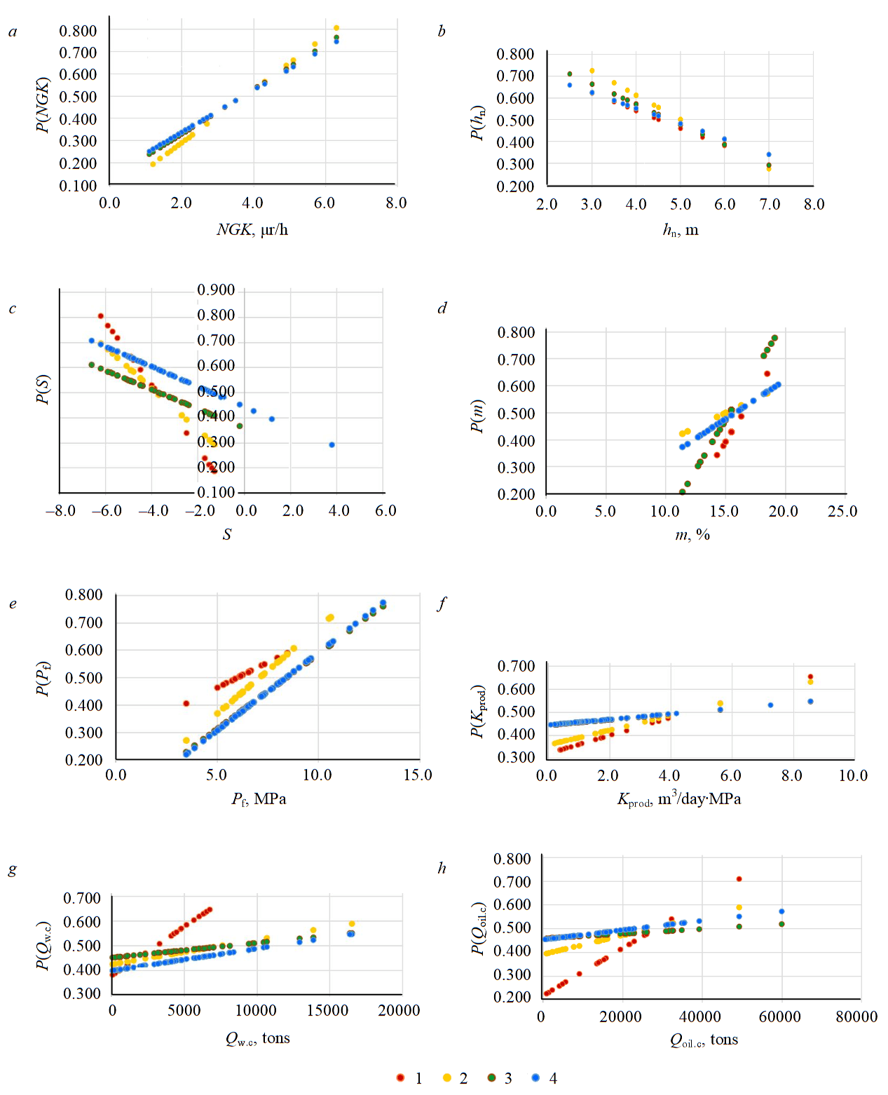
Fig.2. Universal dependencies of geological and technological parameters: a – P(NGK) on NGK; b – P(hn) on hn; c – P(S) on S; d – P(m) on m; e – P(Pf) on Pf; f – P(Kprod) on Kprod; g – P(Qw.c) on Qw.c; h – P(Qoil.c) on Qoil.c
1 – HF 2014-2015; 2 – HF 2014-2016; 3 – HF 2014-2017; 4 – HF 2014-2018
Probabilistic method of data analysis has “transparency”, since in practice it allowed to build probabilistic models and assess the influence degree of indicators on the output indicator Input parameters with different dimensions are compared due to their reduction into a single dimension space.
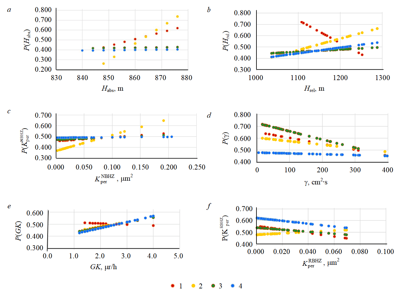
Fig.3. Dependencies of geological and technological parameters:а – P(Habs) on Habs; b – P(Hrel) on Hrel; c – on ; d – P(γ) on γ; e – P(GK) on GK; on
1 – HF 2014-2015; 2 – HF 2014-2016; 3 – HF 2014-2017; 4 – HF 2014-2018
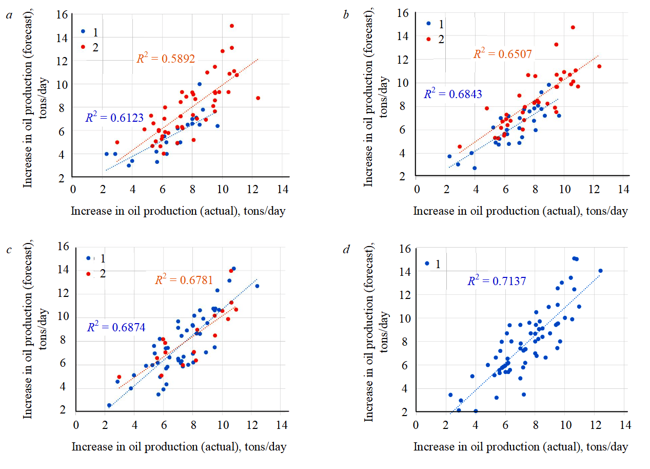
Fig.4. Correlation fields for tutoring samples of wells: а – 2014-2015 (2016-2018 forecast sample, max deviation is 2.9 tons/day); b – 2014-2016 (2017-2018 forecast sample, max deviation is 2.4 tons/day); c – 2014-2017 (2018 forecast sample, max deviation 2 tons/day); d – 2014-2018 (max deviation 1.4 tons/day)
1 – tutoring; 2 – forecast
The most informative parameters influencing the output parameter are determined. The universal dependencies are revealed, ranked by the tgα inclination angle, i.e. the parameters of the indicators that have the greatest influence on the output indicator are determined, and ranked according to this. In the case of tgα ~ 0 geological and technological parameters have no effect and can be neglected. Thus, only the necessary parameters can be determined, which allows further analysis of universal models.
To achieve an increase in oil production of 7 tons/day, the probability must be more than 50 %. Consequently, the values of the criteria for the application of HF technology are located in the range of 0.5-1 units (P(N) ³ 0.5). Thus, P(N) = 0.5 corresponds to the minimum value of the parameter, P(N) → 1 corresponds to the maximum. Universal indicators must meet the criteria for the use of HF technology in a carbonate object В3В4: values of gamma log (NGK) 4.1-6.3 μr/h; drilled-in net oil thickness hn 4.5-2.5 m; skin factor S –1.4- –6.6; porosity coefficient m 16.1-19.4 %; current formation pressure in the well Pf 8.2-13.2 МПа; productivity coefficient Kprod 4.2-8.5 m3/day∙MPa; cumulative oil production since the beginning of well operation Qoil.c, 0682-16523 tons; cumulative water production since the beginning of well operation Qw.c 22810-59802 tons.
Forecasting the increase in oil production
For the purpose of joint use of individual probabilities for geological and technological indicators, the generalized (integrated) probability is calculated [16, 20]. First, integrated probability is calculated for two indicators , at the last step – for eight indicators .
Forecast increase in oil production is calculated for each of the samples with stepwise regression analysis using the values Pint at m from 2 to 8 for geological and technological parameters. Regression equation for a wells sample of 2014-2015 has the following form:
This regression model takes into account the values Pint in combination m = 3, which makes it possible to predict an increase in oil production (for wells in 2016-2018) with a maximum deviation from the actual values of 2.9 tons/day. Similarly, a regression equation is constructed and the forecast is carried out for wells samples of 2014-2016, 2014-2017, 2014-2018.
Figure 4 shows that the calculated values of the increase in oil production correlate quite well with the actual increase in production rates, the values of the correlation coefficients r = 0.58-0.67 for the examined samples of wells. The greatest discrepancy between the forecast and actual data is observed when predicting growth in the period of 2016-2018, the maximum deviation is 2.9 tons/day, in other samples, the smallest deviation is noted. The smallest discrepancy in predicting the increase in oil production rates is in the tutoring sample of wells in 2014-2018.
Conclusion
Main advantages of the probabilistic method of analysis are simplicity and transparency. This method made it possible to significantly reduce the number of free variables, to transfer dimensional indicators into a single probability space.
Description for the construction of individual probabilistic models allowed showing the transparency of this method and the absence of hidden processes. Using tgα it is determined, which of the indicators has the greatest impact on the output indicator. Due to the probabilistic presentation of data for each parameter, the criteria for the application of HF technology at the В3В4 object have been determined, and the permissible probabilistic limits of the technology application have been identified. Analysis of the conducted forecasts allowed determining the reliability of the constructed regression models.
The method is recommended to be used to predict the effectiveness of other technologies application: perforation methods, radial drilling, acid treatment, etc.
References
- Galkin V.I. Kazantsev A.S., Koltyrin A.N. Probabilistic-Statistical Estimation of Different Indicators Used to Determine the Efficiency of a Formation Proppant Hydraulic Fracturing (On the Example of Tl-Bb Terrigenous Formation And V3V4 Carbonate Formation). Oilfield Engineering. 2018. N 2, p. 26-23. DOI: 10.30713/0207-2351-2018-2-26-33 (in Russian).
- Galkin V.I., Ponomareva I.N., Koltyrin A.N. Development of Probabilistic and Statistical Models for Evaluation of the Ef-fectiveness of Proppant Hydraulic Fracturing (On Example of the Tl-Bb Reservoir of the Batyrbayskoe Field). Perm Journal of Pe-troleum and Mining Engineering. 2018. Vol. 18. N 1, p. 37-49. DOI: 10.15593/2224-9923/2018.1.4 (in Russian).
- Galkin V.I., Sosnin N.E. Geological Development of Mathematical Models for the Prediction of Oil and Gas Complex-Built Structures in the Devonian Clastic Sediments. Oil Industry. 2013. N 4, p. 28-31. (in Russian)
- Savchenko P.D., Fedorov A.I., Kolonskikh A.V., Urazbakhtin R.F., Davletova A.R. Method for Selecting Well Candidates Based on the Effect of Fracture Reorientation. Oil Industry. 2017. N 11, p. 114-117. DOI: 10.24887/0028-2448-2017-11-114-117 (in Russian).
- Sosnin N.E. Development of Statistical Models for Predicting Oil-And-Gas Content (On the Example of Terrigenous Devo-nian Sediments of North Tatar Arch). Perm Journal of Petroleum and Mining Engineering. 2012. Vol. 11. N 5, p. 16-25 (in Russian).
- Alimkhanov R., Samoylova I. Application of Data Mining Tools for Analysis and Prediction of Hydraulic Fracturing Efficiency for the BV8 Reservoir of the Povkh Oil Field. SPE Russian Oil and Gas Exploration & Production Technical Conference and Exhibition, 14-16 October 2014. Moscow, Russia, 2014. SPE-171332-RU. DOI: 10.2118/171332-RU (in Russian).
- Anifowose F., Abdulraheem A. Fuzzy logic-driven and SVM-driven hybrid computational intelligence models applied to oil and gas reservoir characterization. Journal of Natural Gas Science and Engineering. 2011. Vol. 3. N 3, p. 505-517. DOI: 10.1016/j.jngse.2011.05.002
- Aryanto А., Kasmungin S., Fathaddin F. Hydraulic fracturing candidate-well selection using artificial intelligence approach. Journal of Natural Gas Science and Engineering. 2018. Vol. 2. N 2, p. 53-59. DOI: 10.33021/jmem.v2i02.322
- Ashena R., Moghadasi J. Bottom hole pressure estimation using evolved neural networks by real coded ant colony optimization and genetic algorithm. Journal of Petroleum Science and Engineering. 2011. Vol. 77. N 3-4, p. 375-385. DOI: 10.1016/j.petrol.2011.04.015
- Gong X., Gonzalez R., McVay D., Hart J.D. Bayesian Probabilistic Decline Curve Analysis Quantifies Shale Gas Reserves Uncertainty. Canadian Unconventional Resources Conference, 15-17 November 2011, Calgary, Alberta, Canada, 2011. SPE 147588. DOI: 10.2118/147588-MS
- Clark A.J., Lake L.W., Patzek T.W. Production Forecasting with Logistic Growth Models. SPE Annual Technical Confer-ence and Exhibition, 30 October – 2 November 2011, Denver, Colorado, USA, 2011. SPE 144790-MS. DOI: 10.2118/144790-MS
- Yu T., Xie X., Li L., Wu W. Comparison of Candidate-Well Selection Mathematical Models for Hydraulic Fracturing. Fuzzy Systems & Operations Research and Management. Springer, Cham, 2015. Vol. 367. P. 289-299. DOI: 10.1007/978-3-319-19105-8_27
- Ma X., Liu Z. Predicting the oil field production using the novel discrete GM (1, N) model. The Journal of Grey System. 2015. Vol. 27. Iss. 4, p. 63-73.
- Mattar L. Production Analysis and Forecasting of Shale Gas Reservoirs: Case History-Based Approach. SPE Shale Gas Production Conference, 16-18 November 2008. Fort Worth, Texas, USA, 2008. SPE 119897-MS. DOI: 10.2118/119897-MS
- McVay D.A., Dossary M.N. The Value of Assessing Uncertainty. SPE Journal. 2014. Vol. 6. Iss. 2, p. 100-110. DOI: 10.2118/160189-PA
- Mohaghegh S., Reeves S., Hill D. Development of an intelligent systems approach for restimulation candidate selection. SPE/CERI Gas Technology Symposium, 3-5 April 2000, Calgary, Alberta, Canada, 2000. SPE-59767-MS. DOI: 10.2118/59767-MS
- Petrakov D.G., Kupavykh K.S., Kupavykh A.S. The effect of fluid saturation on the elastic-plastic properties of oil reservoir rocks. Curved and Layered Structures. 2020. Vol. 7. N 1, p. 29-34. DOI: 10.1515/cls-2020-0003
- Podoprigora D.G., Saychenko L.A. Development of acid composition for bottom-hole formation zone treatment at high reservoir temperatures. Espacios. 2017. Vol. 48. N 38, p. 32.
- Cheng Y., Wang Y., McVay D., Lee W.J. Practical Application of a Probabilistic Approach to Estimate Reserves Using Production Decline Data. SPE Economics and Management. 2010. Vol. 2. Iss. 1, p. 19-31. DOI: 10.2118/95974-PA
- Rahmanifard H, Plaksina T. Application of artifcial intelligence techniques in the petroleum industry: a review. Artifcial Intelligence Review. 2019. Vol. 52, p. 2295-2318. DOI: 10.1007/s10462-018-9612-8
- Sandyga M.S., Struchkov I.A., Rogachev M.K. Formation damage induced by wax deposition: laboratory investigations and modeling. Journal of Petroleum Exploration and Production Technology. 2020. Vol. 10. N 6, p. 2541-2558. DOI: 10.1007/s13202-020-00924-2
- Schapire R.E., Freund Y. Boosting. Foundations and algorithms. Cambridge: The MIT Press, 2012, p. 544.
- Yanfang W., Salehi S. Refracture candidate selection using hybrid simulation with neural network and data analysis techniques. Journal of Petroleum Science and Engineering. 2014. Vol. 123, p. 138-146. DOI: 10.1016/j.petrol.2014.07.036